?Quotes # same information as via the link above13 String operations
13.1 Introduction
Although R is primarily a tool for dealing with numeric data, it is also possible to perform string operations. In this final chapter, we will be practicing string manipulation as a final part of the course.
Tip
A string is a separate data type in R, which you have probably already come across in earlier chapters. Strings are often used for descriptive variables (e.g. the name of a tomato variety like ‘Moneymaker’), but can also more generally be any group of alphanumeric characters, e.g. “abc123_z”. To denote a string we use either '' or "", which are interchangeable, although double quotation marks are preferred.
“String operations” could mean any number of things. For example, concatenating strings together, splitting a character string into a number of parts, replacing a capital letter with a small letter, removing a . character from a name etc.
Once you start working with data more regularly, you will find it is not always in the form(at) you want. String operations are often needed to “get something to work”. Here, we introduce a few of the most common and useful functions for performing string operations, before briefly introducing Regular Expressions.
13.2 R functions for strings
String concatenation with paste()
You have probably already seen this function, or its cousin paste0(). Like many R functions it has a self-describing name, it pastes (strings) together. paste0 pastes with zero spaces between.
Exercise 13.1 (Pasting)
Paste the first 10 letters and the first 10 positive integers together (without any separating space).
Paste the first 10 letters and the first 10 positive integers together, this time separated by an underscore (so “a_1” would be the first element of the resulting vector).
Repeat the first exercise, but this time pasting the first 10 positive integers together with the next 10 numbers (i.e. paste 1 - 10 together with 11 - 20). What is the data type of the output? Hint: use
class()to check.
NoteLeading zeros
If you are assigning names to things like experimental treatments, you sometimes combine character strings with numbers quite naturally, for example “genotype1”, “genotype2”, “genotype3”.
We have already seen how to do this using paste0():
paste0("genotype", 1:3)[1] "genotype1" "genotype2" "genotype3"Suppose we had 20 genotypes in an experiment, we might reasonably call them genotype1 - genotype20:
genos <- paste0("genotype", 1:20)But if we are doing an analysis or plotting the data afterwards, you will notice that the order of the genotypes is not g1:g20, instead they are ordered as follows:
levels(as.factor(genos)) [1] "genotype1" "genotype10" "genotype11" "genotype12" "genotype13"
[6] "genotype14" "genotype15" "genotype16" "genotype17" "genotype18"
[11] "genotype19" "genotype2" "genotype20" "genotype3" "genotype4"
[16] "genotype5" "genotype6" "genotype7" "genotype8" "genotype9" Why do we go from genotype1 to genotype10? Doesn’t R know how to count?
The problem of course is that “genotype1” is now a string, and strings are ordered alphanumerically, meaning that genotype10 comes before genotype2.
We could force the ordering of the genotypes by converting it to a factor with defined levels:
genos <- factor(paste0("genotype", 1:20), levels = paste0("genotype", 1:20))This can be a useful approach if you want a specific order - we already encountered this when trying to visualise the geographic distribution of admixture groups in the same order as the publication (Section 12.10).
Here, we’ll mention a different approach - using leading zeros. There are a number of ways to pad a number with zeros, but here we will only consider one, using the function sprintf(). Have a look at the documentation and see whether you can work out how to add a leading zero so that the genotype names order as we would like. Try this before looking at the Code below.
Code
genos <- paste0("genotype", sprintf("%02d",1:20))

## The first argument starts with % and ends with d (for integers). In between we tell the function to pad with zeros up to 2 digits. If we exceeded 100 genotypes we would have needed "%03d" etc.

genos
[1] "genotype01" "genotype02" "genotype03" "genotype04" "genotype05"
[6] "genotype06" "genotype07" "genotype08" "genotype09" "genotype10"
[11] "genotype11" "genotype12" "genotype13" "genotype14" "genotype15"
[16] "genotype16" "genotype17" "genotype18" "genotype19" "genotype20"Manipulating strings
Suppose we have received a dataset from another researcher where plant heights were measured in centimeters. Unfortunately, the researcher recorded everything in Excel with the letters “cm” following the numbers. We would like to extract the actual heights as a numeric data type so that we can produce a plot.
We can generate an example of such a dataset as follows:
sampledata <- data.frame(Genotype = c("Warwick","Hopkins","Venture","Hopewell","Whitby","Bess"),
Height = c("36.5cm","28.9cm","26.5cm","33.4cm","39.1cm","32cm"))| Genotype | Height |
|---|---|
| Warwick | 36.5cm |
| Hopkins | 28.9cm |
| Venture | 26.5cm |
| Hopewell | 33.4cm |
| Whitby | 39.1cm |
| Bess | 32cm |
Your initial reaction might be to go back to the Excel file you received and delete the “cm” by hand. That might be a good solution in this example, but it would be less good if there were 6000 or 60000 rows in the dataset!
Find and Replace is another option, but this can have unwanted consequences if applied to a whole file (by perhaps deleting “cm” from other columns unintentionally).
Of course, by now you should know that you can do pretty much everything in R! There are a number of ways to achieve this. We will demonstrate the functionality of the functions substr() and strsplit(), using this example.
Extracting a substring with substr()
substr() creates a sub-string of the input, which is exactly what we want here.
Have a look at the function documentation first:
?substrFrom reading this, you should see that you need to know the start and stop position of the characters you want to retain. This causes a slight problem here, as the last height measurement (32cm) was recorded without specifying the decimal place, while the rest were recorded to 1 decimal place. We want to subtract two characters from each string, rather than count from the start (which would go wrong for 32cm if we stopped at the 4th character).
To get around this, we use another (string) function nchar(), which counts the number of characters of a string:
nchar(sampledata$Height)[1] 6 6 6 6 6 4We can tell substr() that we want to stop 2 characters from the end as follows:
substr(sampledata$Height,
       start = 1,
       stop = nchar(sampledata$Height) - 2)
[1] "36.5" "28.9" "26.5" "33.4" "39.1" "32"
NoteRecycling
Notice that in this function, we were able to specify the start position (= 1) only once, and the function understood that we wanted this start position to be used for all 6 heights. This is an example of recycling, which is built into many but not all R functions.
If it were not possible to recycle here you would get an Error (something like argument lengths don’t match), and we would have had to use start = rep(1,6) to repeat the number 1, 6 times (so, make a vector c(1,1,1,1,1,1) as the start positions).
Finally, if we want to get the heights as numeric data, we would wrap the whole expression with as.numeric(), and perhaps add it on to the data-frame as a new column:
sampledata$hgt <- as.numeric(substr(sampledata$Height,
                                    start = 1,
stop = nchar(sampledata$Height) - 2))| Genotype | Height | hgt |
|---|---|---|
| Warwick | 36.5cm | 36.5 |
| Hopkins | 28.9cm | 28.9 |
| Venture | 26.5cm | 26.5 |
| Hopewell | 33.4cm | 33.4 |
| Whitby | 39.1cm | 39.1 |
| Bess | 32cm | 32.0 |
Splitting strings with strsplit()
One of the most basic operations is being able to split a character string at a particular symbol (or combination of characters) such as a “.”, “_” or “-” for example. These symbols often turn up where they are not wanted in datasets, and might need to be removed to proceed with an analysis or operation.
As the function name suggests, strsplit() splits (character) strings at a symbol or combination of characters. You can again check out ?strsplit for the details, but we can apply strsplit() in our example above by asking R to split our heights at the offending characters “cm”:
strsplit(sampledata$Height,split = "cm")[[1]]
[1] "36.5"
[[2]]
[1] "28.9"
[[3]]
[1] "26.5"
[[4]]
[1] "33.4"
[[5]]
[1] "39.1"
[[6]]
[1] "32"The output is a list, and because there was nothing after the “cm”, each list element is of length 1. Splitting a string like “21_583” at _ would result in a vector of length two containing the string before and after _.
A list is not always the most convenient structure for downstream applications, so we can turn it into a vector either using the unlist() function (collapses the list) or, more elegantly, using sapply() with [[ as follows:
sapply(strsplit(sampledata$Height,split = "cm"),"[[",1)[1] "36.5" "28.9" "26.5" "33.4" "39.1" "32" This approach picks out the first element of each list item (the 1 after “[[” specifies this). In another data-set you might want to pick out the second result (for example the number after the _), in which case you would replace the 1 with a 2. Alternatively, you could specify the column name instead of the column number.
Note
You have already encountered the apply family of functions in earlier weeks, for example in week 2 (Section 4.1) when you learned about functions.
The functions apply(), sapply(), lapply() and tapply() are the most commonly-used (mapply() is also available, but I have never used it).
Check out the documentation for sapply(), which is arguably the most-used function in the family:
?sapplyThe Usage section mentions that this function has 3 main arguments, namely X (the input object), FUN (the function to apply to that object) and ... (ellipses, to pass extra arguments to FUN).
In the code above, [[ is actually a function we are applying to the output of strsplit(), and 1 is the extra argument we are supplying to [[1.
13.3 Regular expressions
One extra “programming tool” topic that can get quite complicated but nonetheless is incredibly useful when you need it is Regular expressions. At the very least, just knowing this term may help you successfully Google a solution to a tricky data formatting problem in the future.
Regular expressions are used for character string searches, in a somewhat similar way to Find (and Replace) in MS Word. If you are familiar with Word, you may have noticed that in an Advanced Search, it is possible to “Match case”, only matching capital letters with capitals etc.
Regular expressions can be thought of as a way to describe such matching rules in more detail. Different programming languages have their own syntax for Regular Expressions, including R, which by default uses so-called extended regular expressions (although it is possible to follow the conventions used in Perl for “Perl-like” regular expressions).
A good description of Regular Expression usage in R can be found by looking at the documentation via ?regex.
Associated R functions are grep(),gsub() etc - these are functions that accept regular expressions as matching arguments (usually called the “pattern”, but check function documentation to be sure).
Here we present an example to give you an idea of how regular expressions can be used in R.
We first generate a vector of character strings that mix letters, numbers and an underscore:
set.seed(42) #for reproducibility

vect <- paste0(sample(c("M","Tr","Px","Z"),100,replace=TRUE),
               sample(1:10000,100),"_",sample(1:100,100))

vect[1:10] #show the first 10 elements of vect
[1] "M8274_1" "M9106_17" "M2344_33" "M149_28" "Tr7140_2" "Z5689_31"
[7] "Tr100_8" "Tr2346_80" "M2450_3" "Z91_13" Note that by setting the same seed, you should see the same set of strings as shown here.
We suppose these are genetic marker names, with some prefix depending on the population in which the marker was identified, followed by the contig number and bp position in the contig. We would like to separate out the contig number, the base-pair position and also the prefix itself (so, we do not want to throw away the information, just separate it).
If we performed a string split at the “_“, we could get the base-pair numbers simply enough, but how to separate the letters from the contig numbers? There is no separating symbol like an underscore to split on. To do this, we probably need to use a regular expression approach.
Letters can be represented by “[A-Za-z]” (this considers both upper and lower case letters a match. For only lower case you would use “[a-z]”).
However, we also want to be able to match one or more letters (some of the prefixes are single letters, some are 2 letters). We therefore need to add “+” directly afterwards (otherwise we are asking R to match exactly one letter). So the way to ask R to match any of the prefixes in vect is with the regular expression “[A-Za-z]+”.
Similarly, to match numbers we would use the regular expression “[0-9]+”, which covers (integer) numbers from 0 to infinity (or close enough). Putting this together, we could split up the vector in a couple of steps as follows:
split1.ls <- strsplit(vect, split = "[A-Za-z]+") #split on the prefix letters i.e. remove them

split1.vect <- sapply(split1.ls,"[[",2) #extract the 2nd list elements, like 8274_1 etc

split2 <- strsplit(split1.vect,split = "_") #now split on the underscore, using output split1.vect

contig <- sapply(split2,"[[",1) #extract the contig number

bp <- sapply(split2,"[[",2) #extract the base pair number

prefix <- sapply(strsplit(vect, split = "[0-9]+"),"[[",1) #re-split by number and extract the prefix in 1 go
Try this yourself by copying and pasting the above code into R, and see whether contig, bp and prefix are correct. Notice that in the last line of code, we perform two operations: first splitting vect at the numbers, and then pulling out the first element of the resulting list. As you use R more, you will find that it becomes easier to build up a few operations in a single line by nesting bits of code within other code, passing the output from one function as the input to the next function wrapping it.
So we read (base) R code not so much from left to right, but from inside to out (and this is also how the code is written, from inside out). This is often presented as one of the main arguments for using tidyverse syntax and piping, making it easier for others to read as well by following a natural textual order from left to right and top to bottom2.
If you are unsure about how part of the code works, just highlight that part of the code (e.g. strsplit(vect, split = "[0-9]+")) and Run that (Ctrl + Enter) to make sure it works.
A more elegant solution would be to split the regular expression into “groups” (defined using round brackets), and access each of these groups in turn using the gsub() function:
myregex <- "([A-Za-z]+)([0-9]+)(_)([0-9]+)" #here we define 4 "groups", each contained by round brackets

prefix <- gsub(myregex, replacement = "\\1",vect) #replace the whole string with the match from group 1
contig <- gsub(myregex, replacement = "\\2",vect) #similarly, group 2 (denoted \\2) is the contig

bp <- gsub(myregex, replacement = "\\4",vect) #we skipped group 3, the underscore
If you want to do all this in a single line of code, you will need to install the stringr package which extends the capabilities of R a bit further in this direction:
install.packages("stringr")

result <- stringr::str_match(vect,"([A-Za-z]+)([0-9]+)(_)([0-9]+)")

head(result) #show the first 6 rows of the result
[,1] [,2] [,3] [,4] [,5]
[1,] "M8274_1" "M" "8274" "_" "1"
[2,] "M9106_17" "M" "9106" "_" "17"
[3,] "M2344_33" "M" "2344" "_" "33"
[4,] "M149_28" "M" "149" "_" "28"
[5,] "Tr7140_2" "Tr" "7140" "_" "2"
[6,] "Z5689_31" "Z" "5689" "_" "31"Each of the groups are given in a separate column, along with the original string that needed to be split (useful for comparing to see it worked).
Exercise 13.2 (Practicing string manipulations)
- Using the
substr()function, remove the starting letter from elements of the vectorv:
v <- c("M1234567","N23456","O345678","P4567","Q567890","R67")- Extract the words “COVID” and “SARS” from the vector
cov, ie. extract the word before the first dash symbol:
cov <- c("COVID-19","SARS-CoV-2")- Standardise the vector ‘test’ below to have an underscore between the prefix letters and numbers (so, all elements having the form Na_123 for example):
test <- c("Br 10992","Fe 9056","Io 999","C 14","Ka 167")- Convert the following string into lower-case letters only:
book_string <- "Down and out in Paris and London. Ed. Penguin Books Ltd."As usual, please attempt these exercises yourself first! If you are unable to complete them after a reasonable attempt, a sample script will be made available on Brightspace week 4. If it is not yet visible, please raise your hand.
13.4 Unexpected data formats and readLines()
As a final topic in this section, we will briefly look at what to do when the data you would like to work with is not loading properly.
You have been practicing the data-science cycle during the past four weeks, but occasionally data is not in an easy-to-load format. This can often happen with older datasets that were prepared with older (and perhaps obsolete) software in mind, each with its own syntax (you’ve already encountered some syntax differences in this course - for example, comments in R are preceded with a hashtag (#), while in markdown files hashtags denote Headers!).
I was recently asked by a former colleague to advise on R software packages for QTL mapping. The datafile the researcher wanted to use was downloaded from TAIR - Arabidopsis again! - and was in JoinMap format (if you are interested, you could visit Kyazma’s website).
Looking at the file in a text editor shows the difficulty in accessing the data in R:
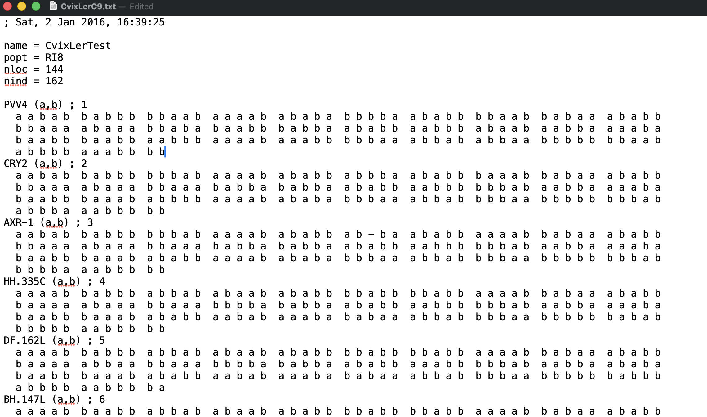
The initial line in the file is preceded by “;” denoting a comment, followed by a time-stamp. The next line is blank, there are then 4 lines with some descripive information on the name of the population, the population type, the number of loci and individuals, followed by another blank line and then the marker information.
If we try to read this data in using read.table() or read.csv() we will get an error!
data <- read.table("CvixLerC9.loc")Error in scan(file = file, what = what, sep = sep, quote = quote, dec = dec, : line 2 did not have 6 elementsThe end of this rather long Error message is informative - line 2 did not have 6 elements. The function read.table() expects data to be in a sqare format, not with unequal numbers of potential columns from one line to the next.
If you dig into the documentation for the function, you can see that there is an argument skip that we might use, skipping over perhaps the first seven or eight lines lines. Let’s try it…
data <- read.table("CvixLerC9.loc", skip = 7)Error in scan(file = file, what = what, sep = sep, quote = quote, dec = dec, : line 1 did not have 50 elements## or maybe:
data <- read.table("CvixLerC9.loc", skip = 8)Error in scan(file = file, what = what, sep = sep, quote = quote, dec = dec, : line 4 did not have 50 elementsread.tables() keeps getting stuck. Not only are there unequal numbers of elements, the data has been organised in chunks of 50 data-points (a or b denoting allele a from parent 1, or b from parent 2). With 162 individuals, we are left with an overhang of 12 elements after the first 150..
How can we proceed? Do we throw out the data? No need! R has this covered, namely with the function readLines()!
attempt1 <- readLines("CvixLerC9.loc")

dim(attempt1)NULLattempt1[1:10] [1] "; Sat, 2 Jan 2016, 16:39:25"
[2] ""
[3] "name = CvixLerTest"
[4] "popt = RI8"
[5] "nloc = 144"
[6] "nind = 162"
[7] ""
[8] "PVV4 (a,b) ; 1"
[9] " a a b a b b a b b b b b a a b a a a a b a b a b a b b b b a a b a b b b b a a b b a b a a a b a b b"
[10] " b b a a a a b a a a b b a b a b a a b b b a b b a a b a b b a a b b b a b a a b a a b b a a a a b a"attempt1 is a character vector, not something that you usually have to work with as genetic marker data, but here it is the first step at getting the data into R. A number of string operations will be necessary to extract the genotypic data and convert it into a numeric matrix.
This is left as a final exercise to practice on (slightly advanced level). A sample script to complete this exercise will be made available via Brightspace after a reasonable attempt has been made by most students.
Exercise 13.3 (Converting output of readLines) The steps described below provide a suggested approach to solve this problem. You may think of another way, which is also fine.
Use the
readLines()function to read in the .loc file. Check how many lines have been read in.Use
grep()with a suitable “pattern” to find the lines with the marker names.Apply a suitable string splitting approach to extract the marker name without the extra information or comment (e.g.
PVV4 (a,b) ; 1should be simply bePVV4etc.)Use the marker name information to also work out the line numbers of where the genotypic data starts. Hint After each markername there is always 4 lines of marker information.
Convert the dataset to numeric format in a matrix, with 0 in place of ‘a’ and 1 in place of ‘b’. Have markers in rows and individuals in columns.
Use the marker names as the rownames of the matrix.
Double-check the data for characters other than ‘a’ or ‘b’, and make sure these have been correctly handled in the conversion step.
13.5 Assignment for week 4 code peer-review
Finally, the following exercise needs to be submitted by the end of the day today, in .qmd format. Please check that the file actually Renders correctly before submitting!
Note that you are not provided with a markdown / quarto template for the assignment. This means you will also need to pay attention to the layout and structure of the document yourself.
To get started, create a new .qmd file in R for your work. Choose suitable section headings (e.g. using question numbers given below) for each sub-question.
Exercise 13.4 (Week 4 (peer-review) assignment)
Download the data file (“week4_assignment.dat”) available from Brightspace week 4. Read it into
Rusing a suitable function.Describe the dataset along the following lines:
What is the structure of the dataset (data types in each column)
What is the dimension of the dataset
How many genotypes
How many replicates
Presence of missing values in each column.
Use appropriate string operational function(s) to extract numeric values from the height and biomass columns.
Make a scatter plot of the height (x axis) versus biomass (y axis), colouring the points by genotype. If you like, choose a colour-blind friendly colour palette.
Fit an appropriate linear model with biomass as the response variable and height as the explanatory variable, allowing for separate fitted lines per genotype.
Check the residual plots after model fitting. Do you find evidence of outliers in the data? If yes, remove these data points from the dataset and re-run the model. How do the residual plots look now?
Calculate the correlation coefficient between plant height and biomass. Compare this to the \(R^2_{adj}\) from the fitted model. Can you account for the discrepancy between these numbers?
You can submit the completed .qmd file via Brightspace for feedback on Thursday. Please do so before Wednesday night 23:59.
Note that I have deliberately written
[[and not[[()when referring to the function[[here. This goes a bit against convention: elsewhere in these notes functions are written likeplot()to explicitly refer to the functionplot.↩︎As an enthusiast of
base R(for its stability, few dependencies etc), I find the readability argument somewhat spurious. Personally, I primarily write code for a computer to read. If I want to write something for a human to read, I document my code via comments, as should you!↩︎