### here add the code to read the data3 Your digital notebook
3.1 Your digital notebook
Introduction to day 3
Today we will continue with goal 1 (Built basic knowledge on using R and R studio) and goal 3 (Apply common statistical tools for inspecting and analyzing data). We will also start with goal 4 (Be able to document your code in a clear & concise way). You will find out that we’ve already covered this by requiring you to write a script. Now we’ll add one more layer to it, the notebook.
New today, is that you get an assignment. In this assignment, you are expected to go over goal 5 [Apply the data-science cycle (load, inspect, clean, analyse, present)]. Also, this is not new, we’ve been doing it for the past two days.
As on the previous days, we will be making use of a real data-case.
TipPlant growth impairment by nematodes.
You already know that plant susceptibility to nematodes is a complex trait, with a lot of variation in susceptibility between individuals of the same species. This variation also exists for the dose-response relation between plants and nematodes. The data you will be using today is derived from a study by Jaap-Jan Willig, who used a camera platform to track the growth of 960 A. thaliana plants simultaneously1.
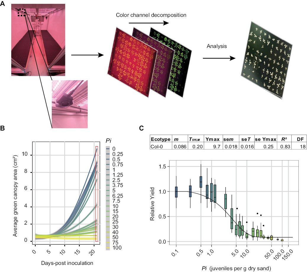
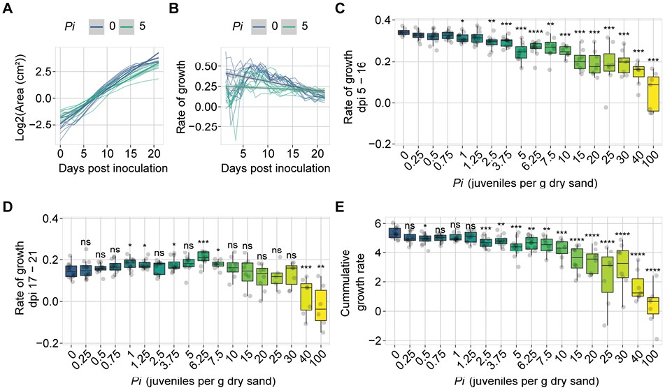
The goal of this research was to develop a platform that allowed us to track in real-time plant growth under below-ground biotic stress caused by nematode infection. Doing this experiment, we identified a compensation response where, at low levels of infection, plants perform better than in uninfected conditions.
Set up your R environment
For the basics of setting up your environment, you can check Chapter 1.
Quarto markdown
The use of a markdown document
The last two days you have been working with .qmd files (Quarto markdown). This is a flavor of markdown, which is a markup language that relies on simple text to produce a layout of a document. As you have a lab-journal for experimental work in the field, greenhouse, or laboratory, a markdown notebook is useful to have when writing code.
The Quarto markdown file you make today for the assignment, should be handed in on Brightspace today, before the deadline. You hand in the .qmd file. Your reviewer will go through the file and check if it renders and whether your conclusions are correct.
Exercise 3.1 (Make your own markdown file) In RStudio go to File > New File > Quarto document…
Based on the documents provided last two days (Chapter 1 and Chapter 2), make your own markdown file. Include meta information (title, name, registration number) and headings for: setup of the R environment (working directory, packages), and the five steps in the data analysis cycle (see Chapter 1).
You can choose whether it renders a .html or a .pdf document. For now, settle on .html, this typically renders well and does not require many additional programs. You probably will need pandoc.
You can find general tips on how to write in markdown in Appendix QMD notebook cheatsheet.
Typically, when you make a markdown file, you can make errors. RStudio tries to make you aware of these errors by putting a notification at the line numbers. But some errors you only catch when you render the document. Or when you run code line-by-line.
Many errors were made by me - and the other teachers - in building the book you are now reading. Do ask us about our frustrations in working with R.
3.2 Analysis of plant-growth data
Today we want to cover one more aspect of data analysis, namely including the fit of a simple model into a plot. In this case, we will use some plant-growth data. And to be precise, we will use the linear part of the growth curve. It is perfectly possible to fit a growth-model within R, but we want to start a bit simpler with an actual linear curve. you can find the data for this assignment via the fileshare on Brightspace. You need the general file under day 3, not your personal dataset for the code-review assignment.
Exercise 3.2 (Loading data into R) Load the data using load(). We have not used this function before. Use ?load() to figure out how this function works.
Note that the name of the object you loaded into memory is not the same as the name of the file you have on your hard disk. The reason is that the filename is inherited from my R-environment. Also note that this can be a major source of annoyance; namely we have been using object name pheno_data consistently. If you were to run load(), that would also mean you overwrite any other file with that name in the R environment.
Up till now, we have been avoiding talking about many of the programming aspects of working with R. But, grasshoppers, I’m afraid it is due.
There are some things you probably noticed by now: any wrong wording, comma’s or other ‘unintended mistakes’ from your side are immediately recognized by R and rewarded with an ‘error’. There are also so-called ‘warnings’. The difference is that ‘error’ results in code that does not work (e.g. you will not get the specific calculation/processing executed) and a ‘warning’ means that you might have done something that was not intended (but you will get output). Next week in Chapter 5 we cover this more thoroughly.
The most important step in data-analysis is checking after an operation. Make sure that what you did was what you intended and that what comes back is correct. How often have we, your teachers, not wept when we ‘quickly’ skipped this and found out that the output we got was incorrect.
There are some general measures you can take to reduce risks:
- Always start with a clean environment. At exit, do not save the environment, but start afresh. This ensures that you know which packages you loaded, which files you need to collect, which variables you need to define.
- When writing a pipe (
%>%) or any complex set of operations, check each step individually. Was the outcome of your function as intended? - Do a pilot. If you run a calculation that takes a long time, run it on a small subset of your data and thoroughly check the output.
- Know what you do, especially with statistics. Always visualize the outcome of the analysis if you can. Otherwise it might be that you take a trip into statistical winter-wonder land.
- Be wary of the class factors. Factors are indexed sets of data. If this indexed set of data is a number, the number on which the calculation is performed is the index number, not the actual number you see. In this case, you need to transform the factor to an actual number. You can check if this might be a problem using the function
class().
Inspecting data
Using functions
Inspect the data using the same functions as in Chapter 2. Also, these functions you can find in Appdix Base R cheatsheet.
Code
    head(pheno_data)
    tail(pheno_data)
    summary(pheno_data)
    length(pheno_data)
    ncol(pheno_data)
    nrow(pheno_data)
    dim(pheno_data)
Exercise 3.3 (Inspecting data) Answer these three questions:
What does the
head()function tell you about an object?Similarly, what does the
tail()function tell you about an object?If you would not know this, what is the command you could execute within the R console to find out?
Cleaning and preparing the data
Not needed here today. We keep this heading in for completeness though.
Analyzing
Now the fun starts. We pick up on our old friend cor(). To determine which kind of correlation we need to perform, we need to figure out the statistical distribution of the data.
Normal distribution
Same as before, let’s figure out whether the data is normally distributed. If you don’t know the two tests anymore, check back at Chapter 2.
    ###Use the graphical method

    ###Use the statistical method
Exercise 3.4 (Does the data follow a normal distribution?) You now conducted two types of analyses that tell you whether the data is normally distributed. What is your assessment, is it normally distributed?
Correlation analysis
Yesterday we conducted an analysis of correlation using the cor() function. There is actually another way to conduct this type of analysis, namely using a linear model with lm(). The advantage of this method is that we will get a slope and an intercept.
We can use the function summary() to get the fit of the model.
    data.test <- pheno_data

    ### here the linear model is done
    tested <- lm(value~dpi,data=data.test)

    ### use summary to get the fit
    summary(tested)
The summary() function is a very versatile function, that can generate outputs from many objects. In this case, it presents the analysis from the linear model, which in essence fits a correlation line. The Estimate for the intercept of that line (-2.97528) and the slope (0.50663) are reported. Also the fit of the model (the Adjusted R-squared: 0.8274) and of the parameters. For instance, there is a significant correlation between day post infection (dpi) and the leaf area (value); p < 2e-16.
Presenting
Scatter plot
Now, let’s make a proper plot of correlation. Of course, you can find instructions in both Chapter 1 and Chapter 2. Also, check Appendix GGplot cheatsheet.
    data.plot <- pheno_data

    ###I'm getting the statistics here
    statplot <- broom::tidy(summary(lm(value~dpi,data=data.plot)))

    p1 <- ggplot(data.plot, aes(x = dpi, y = value)) +
          geom_point() + geom_smooth(method = "lm") +
          theme_bw() + annotate("text",
                                x=10,
                                y=max(data.plot$value),
                                label=paste("p =", signif(statplot$p.value[2], 2)))

    p1
Exercise 3.5 (Is the plant-growth correlated with time?) What is the biological interpretation of the correlation you calculated and observed?
What does the intercept represent?
What does the slope represent?
Is a linear model a good fit for plant growth in general?
3.3 Assignment for code-review week 1
The assignment
Via the fileshare on Brightspace, you can find your dataset for the code review. Everyone of you has their own folder, with their own dataset. This means that the conclusions you draw will be based on your individual dataset. We expect that you hand in a .html file generated using a Quarto Markdown (QMD) file you wrote yourself in R. Within the .html file you provide the code to:
- Setup of the R environment
- Load the data
- Inspect the data
- ‘Clean’ the data
- Analyse the data
- Present the data
Also, you should provide a conclusion about the biological interpretation of the data. The exercises below take you through the assignment step-by step. Make sure that for the R steps you include code chunks. If you print figures or execute functions within these blocks, the output will be included in the .html.
Do not wait untill you are finished to make the first render. At the very start, when your file is still pristine (e.g without code chunks but after adapting a .qmd file from Chapter 1 or Chapter 2), do a check on whether it renders correctly. You render the document by hitting the ‘Render’ button on top of the top-left pane in RStudio.
Note that in day 1 and day 2 the parameter eval is set to false in the yaml header (this is the text at the start of the document between the --- and ---). This means that in the .html generated, none of the code blocks are executed. This is a good option to prevent R coding errors from rendering the document. However, if you want to include a figure, you need to set this option to true within that code-chunk #| eval: true.
If you need more tips in general on QMD, check Appendix QMD notebook cheatsheet.
Exercise 3.6 (Setup of the R environment) Set the working directory and install and activate the required packages to run the code within the file.
While going through the exercises, you might encounter steps requiring you to install additional packages. Simply add them to this section of the code one-by-one. You help yourself by being explicit about which package you use (e.g. dplyr:: or tidyr::).
Exercise 3.7 (Load the data) Load the two data files into the R environment using the appropriate read function. Make sure that your name is included here, so the reviewers can check if your code works. That way your reviewer can find your datafiles.
The data consists of the growth rates of A. thaliana Col-0 when inoculated with either of two plant parasitic nematodes1. The two nematode species tested are the beet-cyst nematode Heterodera schachtii and the root-knot nematode Meloidogyne incognita. Within your personal folder you find the data of the experiment conducted at a particular infection density (Pi) in nematodes g^-1. The measured trait is the day-by-day growth rate, measured between two consecutive days post infection (dpi). For instance between day 2 and day 3. The dpi within the data file would be 2.5 in that case. This data is given per plant.
Exercise 3.8 (Inspect) Inspect the data using functions (no plot required). Based on the output indicate which bind function you need to use to combine the two objects into one.
Exercise 3.9 (Clean; combine) Use a ‘bind’ function to combine the two objects into one.
We covered the bind functions in Chapter 2) when combining the four objects.
Exercise 3.10 (Analyse) Compare growth rates of the A. thaliana plant when infected with either H. schachtii or M. incognita, analyse whether these differ using a test that does not assume a normal distribution. Report at least the p-value.
We do not ask you to check for normality for this assignment, as that dataset overall is not normally distributed, we give you that your subset is also not. Note that in the paper We deal with this by using a non-parametric test as well1.
Exercise 3.11 (Present) Make a ggplot2:: boxplot showing the two nematode species on the x-axis and the growth rate on the y-axis.
We covered the boxplot function in Chapter 1) in the presentation section. Also, you can find how to in Appendix GGplot cheatsheet.
Now you have analysed the difference in growth rates between the two species at a particular density at a particular day of the experiment. Now it is time to draw conclusions.
Exercise 3.12 (Interpret) What is the biological interpretation of the boxplot and the wilcoxon-test p-value?
Once you have worked through all these excercises related to the assignment, you can render the .html file. Check the file (is everything included?). If you run into errors, the ‘Background Jobs’ window will indicate where the rendering has halted.
How to do code-review
During code-review, we try to establish if the code that is written:
- is well-organized
- is well-documented
- properly used
- works
Next to that, we also check whether the conclusions drawn from the analysis and figure are valid.
How to give peer-feedback
You need to review 2 coding assignments of other students within the course. Your teachers will check your feedback. In the first week, you will get an indication from us whether you give sufficient and clear feedback. You need to get a ‘pass’ for the assignments in week 2-4.
What is feedback?
Feedback literally means ‘giving back’. It is not an euphemism for criticism. Rather, feedback can be described as: information regarding the way my message or behaviour (or coding and interpreting the outcome of data-analysis in this case) has been received and interpreted. Feedback stimulates you to think about and implement possibilities to improve.
Feedback is critical for your own improvement. Peer feedback relies on giving and receiving feedback. Receiving feedback allows you to develop your competences and skills. Well-given feedback can help you asses your strengths and weak points, and allows you to address the weak points from the basis of your strengths. However, giving feedback also ask you to be critical and recognize certain aspects of data analysis, which you can implement again in your own process of analyzing data in R.
How to give feedback
When giving feedback it is important to:
- Balance your feedback. Mention both positive and constructive aspects (Tops and Tips). It is equally important to know your strengths, as it is to know your weaknesses. Moreover, it is motivating to receive positive feedback.
- Be specific. Feedback is not helpful to the receiver when the feedback is not specifically formulated. Comments such as: “I think it is bad code and it needs revision” does not tell the receiver why it is a bad code. Instead, “I think you arrive at your result in more steps then necessary, I suggest you use function x instead of function y and function z” is much more helpful.
- Connect concrete suggestions for improvement when providing constructive feedback. This can be quite challenging, and requires you to place yourself in the shoes of the someone else. This is very helpful for the receiver, as they receive help on how to improve.
- Provide examples. Link your feedback to specific pieces of code or sentences in the document. In Feedbackfruits you can highlight text and make comments.
- Formulate your feedback to what you observe (objectively) in an open way (without judgement or premature conclusions). For instance: “I noticed that you used the same object name for two different datasets, did you do this for a certain reason?” You can also describe the effect it has on you: “For me, it would be more logical if you use readxl::read_xlsx() to load an .xlsx file instead of read.delim().”
- Do not generalize. Avoid words like always/never in your feedback e.g. “You always forget to indicate which package a function comes from…”
Well organized code
There are many ways in which you can write well-organized code. What all have in common is consistency. Here, I teach you a way of doing this. These are the rules that I generally follow. I would like to stress that these are guidelines. These guidelines help others to read and understand your code. However, they also help you when you need to re-use or re-run your code.
Check:
- Are clear section-level headings used?
- are hierarchies indicated with a tab?
- from non-base R functions, is the package indicated (e.g.
dplyr::)? - do objects have a clear, understandable, name?
Well documented code
When writing code, leave comments. Especially when you’re doing something new / special this is very helpful to you in the future. But also to others that will check or even use your code. It can be very handy to indicate why you use a particular function for instance.
Check:
- Are comments included in the code?
- Above code chunks, is there an explanation of what is done and why?
Properly used code
This checks whether the functions are used as intended. For instance, you can run a correlation analysis on numbers that are of class factor (check this by using class() on a vector/data frame column). However, correlations should be done using actualy numbers is.numeric() should return TRUE. Another example is whether the correct statistical test was used given the data?
Check:
- Are the correct functions / inputs used?
Working code
Check:
- can you run the code and get the same output?
The Biological interpretation
Do you agree with the biological interpretation given? Note that all of you have different days and Pi’s to compare. Thus, the conclusions will probably differ amongst yourselves!
Some reading
Yesterday you might have been convinced that a hypothesis is a liability2, today you may convince yourself otherwise. There is a nice critique written of the provocative paper you read yesterday. The authors in the paper ‘The data-hypothesis relationship’ will convince you that a hypothesis is not such a bad idea after all3.