# Do plant species with a high specific leaf area have a high leaf nitrogen content?
cov(corre_continuous$SLA, corre_continuous$leaf_N, use='complete.obs')
[1] 11.78539In this chapter we cover a fundamental approach for comparing two variables: correlation. Calculating correlation is often an important part in the data analysis pipeline (Tip 1). Just like summary statistics, correlation can be relevant in both the inspecting and analyzing parts of the pipeline. Since correlation is about comparing things, it is critical for the interpretation of a correlation analysis that it is clear what is being compared.
We first introduce the concept of co-variance, from that we derive linear and non-linear correlation measures. We then briefly discuss statistical testing of correlation measures, and we finish with testing and interpreting a correlation analysis (and how to use correlation in building an argument).
In Section 4.2.2 we introduced the concept of variance. By calculating the variance you can answer the following question: how much do individual observations differ from the mean? In this chapter we are interested in comparing two variables, and so we generalize the notion of variance to co-variance. By calculating the covariance you can answer the following question: if one variable variable varies by some amount, how much does my second variable co-vary? In other words: if one variable is high, is my other variable high as well? In a concrete example: do plants that have a large specific leaf area also have a high leaf nitrogen content?
The mathematical derivation for the covariance is relatively straightforward and directly builds on the definition of variance (Equation 6.1).
\[ Variance(X) = \frac{1}{N}\sum_{i=1}^{n}{(\mu-x_i)^2} \tag{6.1}\]
We start by writing the squared difference from the mean as explicit multiplication (Equation 6.2).
\[ Variance(X) = \frac{1}{N}\sum_{i=1}^{n}{(\mu-x_i)(\mu-x_i)} \tag{6.2}\]
Next we swap out one of the difference terms with the difference from the mean of another variable. Note that we use the respective means for the two variables: \(\mu_x\) and \(\mu_y\) (Equation 6.3)!
\[ Covariance(X, Y) = \frac{1}{N}\sum_{i=1}^{n}{(\mu_x-x_i)(\mu_y-y_i)} \tag{6.3}\]
The R language has a built-in function for computing the covariance:
# Do plant species with a high specific leaf area have a high leaf nitrogen content?
cov(corre_continuous$SLA, corre_continuous$leaf_N, use='complete.obs')[1] 11.78539Exercise 6.1 (Comparing variance and covariance) The formulas in Section 6.1 derive how covariance is a generalization of variance. In this assignment you will verify this empirically using R’s built-in var and cov functions. For a variable of your choice, compute the it’s variance, and the covariance of that variable with itself. Compare the outputs. How do you explain this? Hint: compare Equation 6.3 with Equation 6.2.
Exercise 6.2 (Interpreting the units of covariance) As discussed in Section 4.2.3, the units of variance are the square of the units of measurement. Verify how you can derive this from the mathematical formulation of the variance (Equation 6.1). Next, describe what the units of covariance are. How interpretable do you think the units of covariance are? Hint: identify what the units of the two separate elements of the product term inside the sum are, and compare those to the units of measurement.
In Section 4.2.3 we discussed how the standard deviation solves a problem of the variance: it expresses the units in which we express variation in the same units as the mean and the original observations. Correlation solves a similar problem that occurs with the covariance, but in a slightly different way. In Exercise 6.2 you worked on the units of covariance, and from that is should become obvious that it is not straightforward to transform the units of covariance into the original units of measurement. In addition, the covariance can take on values in the range -inf to +inf. The pearson correlation coefficient solves some of these issues: it normalizes the covariance to be restricted to the range -1 to +1, and as a side-effect is a dimensionless quantity.
To normalize the covariance, the pearson correlation coefficient divides the covariance by the product of the squared variances (Equation 6.4).
\[ PearsonCorrelationCoefficient(X,Y) = r{X,Y} = \frac{Covariance(X,Y)}{\sqrt{Variance(X)}\sqrt{Variance(Y)}} \tag{6.4}\]
This is also often expressed in terms of standard deviations \(\sigma\): \[ r_{X,Y} = \frac{Covariance(X,Y)}{\sigma_X \sigma_Y} \tag{6.5}\]
The pearson correlation coefficient \(r\) has a few useful properties that help interpretation.
-1 to +1: correlation coefficients of 1 (either positive or negative) indicate a perfect relationship (in other words, all values are exactly equal). A correlation coefficient of 0 indicates no relationship.Exercise 6.3 (Verify the calculation of the pearson correlation coefficient.) Equation 6.5 describes the pearson correlation coefficient in terms of covariance and standard deviations. Pick two variables of your choice in the corre_continuous dataset and verify the output of cor() with calculating the coefficient yourself using cov() and sd().
Exercise 6.4 Since the pearson correlation coefficient describes a linear relationship, it is relatively straightforward to draw this relationship as a straight line in a scatterplot. Using ggplot, create a scatterplot of your two variables of interest with geom_point and add the correlation line using geom_smooth. Make sure to use method = 'lm' for geom_smooth. What is the relationship between the pearson correlation coefficient and the line you’ve drawn?
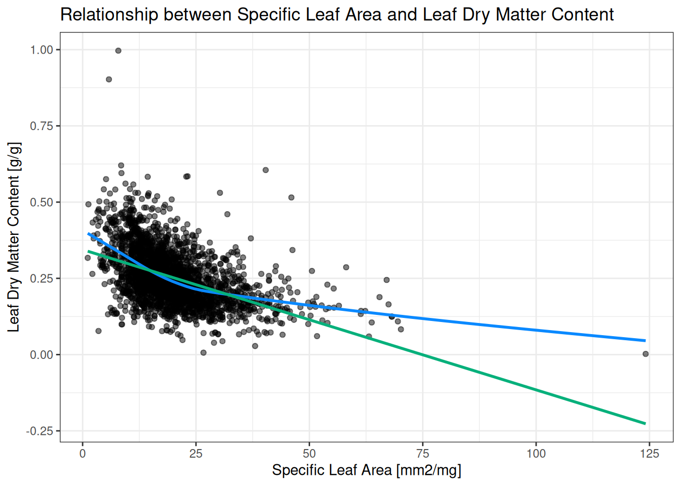
Not all real data is best described by a straight line (Figure 6.1)! We will not go into too much detail on how to express non-linear relationships here (there are many options, most are outside the scope of this course). However, a relatively straightforward modification of the spearman correlation coefficient makes it somewhat suitable to express non-linear relationships. The spearman correlation coefficient is a non-linear correlation approach that simply calculates the pearson correlation coefficient on the ranks1 of the variables. In doing so, spearman correlation effectively ignores the magnitude of the differences in a variable: big jumps are just as important as small jumps. Spearman correlation keeps most of the properties of pearson correlation (Note 6.1 ) except one: the relationship is no longer linear, but instead monotonic: the variables consistently increase or decrease together, without requiring a straight-line relationship.
Exercise 6.5 (Verifying the spearman correlation coefficient) Section 6.3 describes how non-linear spearman correlation is a simple modificiation of pearson correlation. Verify this is true: you can get the ranks of a variable by using the rank() function. Pick two variables of your choice, and compare spearman correlation (cor() function with method = spearman) to pearson correlation on the ranks.
Exercise 6.6 (Interpreting the difference between Spearman and Pearson correlation) For two variables of your choice, compute both the spearman and pearson correlation coefficient. Are they different? How different are they? What do you think this means?
Exercise 6.7 (Computing many correlations on the same dataset) For datasets with multiple quantitative variables, a straightforward question is to ask ‘which variables are correlated with each other?’. The built-in cor() function makes use of vectorization (See Section 4.3.3) to make this a straightforward question to ask.
Select all numeric columns of the grassland_traits_environment dataset:
numeric_columns <- sapply(grassland_traits_environment, is.numeric)
grassland_numeric_df <- grassland_traits_environment[numeric_columns]
Compute pairwise correlations of all variable pairs:
cor(grassland_numeric_df, use = 'complete.obs')What does the output look like? How do you interpret all these numbers? What does use = "complete.obs" do (Hint: check the documentation with ?cor)?
From Note 6.1 it has become clear that a correlation coefficient of zero indicates no relationship. But when do we call a non-zero correlation coefficient sufficiently large to indicate a significant relationship? This is a question that typically lends itself for a statistical approach! In Section 6.4.1 we will not go into too much detail, but a brief description of how significance testing for correlation coefficients work is necessary to interpret results. Once we have established how to determine which correlation coefficients can be seen as statistically significant, we ask the question “how to interpret a significant correlation?” in Section 6.4.2.
The main points for statistical testing of correlation coefficients are bundled in Note 6.2.
To test whether a correlation coefficient is (statistically) significantly different from zero, we take into account three things:
For Pearson correlation the test looks as follows: we compute a t-statistic based on sample size \(n\) and correlation coefficient \(r\), and we compare the t-statistic to a t-distribution to get a p-value. Approaches for other correlation coefficients are similar in nature, but differ in details. \[ t = r\sqrt{\frac{n-2}{1-r^2}} \tag{6.6}\]
From Equation 6.6 it can be observed that a large sample size \(n\) will always lead to a large test statistic \(t\), which in turn will always lead to a low p-value. Table 6.1 provides a few examples of which correlation coefficient will be significant at various sample sizes.
| Sample size | Smallest |r| that is significant |
|---|---|
| n = 10 | ≈ 0.63 |
| n = 30 | ≈ 0.36 |
| n = 100 | ≈ 0.20 |
| n = 1000 | ≈ 0.06 |
The take home message here: A correlation is significant when the data provide enough evidence that the true association is not zero. This depends more on sample size than on the strength of the relationship!
Exercise 6.8 (Exploring Anscombe’s dataset) In this assignment you’ll explore the limitations of summary statistics and correlation. Understanding these limitations is very important when analysing real datasets. To make the limitations very explicit, you will use a artificial dataset designed in 1973 by statistician Francis Anscombe. There are four pairs of observations in this dataset, so it’s often referred to as ‘Anscombe’s quartet’. You can load the dataset into your R session with data(anscombe), the corresponding dataframe will be called anscombe.
summary() function. What do these look like?X and Y, check both Pearson and Spearman. What do these look like?After calculating the summary statistics, let’s take a look at a plot of these four pairs of observations. Copy-paste the code below2 and run it in your R session. What do you observe? How does this affect the interpretation of the summary statistics and correlation coefficients?
# Plotting anscombes quartet
library(ggplot2)

# Load the built-in dataset
data(anscombe)

# Reshape to long format
anscombe_long <- data.frame(
  x = c(anscombe$x1, anscombe$x2, anscombe$x3, anscombe$x4),
  y = c(anscombe$y1, anscombe$y2, anscombe$y3, anscombe$y4),
  set = factor(rep(1:4, each = nrow(anscombe)))
)

# Plot
ggplot(anscombe_long, aes(x, y)) +
  geom_point(size = 2) +
  geom_smooth(method = "lm", se = FALSE, color = "red") +
  facet_wrap(~ set, ncol = 2) +
  labs(
    title = "Anscombe's Quartet",
    x = "x",
    y = "y"
  ) +
theme_minimal()The main interpretation of finding a (significant) correlation between two variables, is that these two variables are somehow related. This might seem obvious at first, but there are a few subtle nuances that are important to realize that might lead to over interpretation when ignored. The most important nuance of correlation, is that it is not causation (See Warning 6.1).
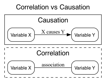
Correlation describes that two variables are related, it does not tell you why the variables are related. In many cases you will be interested in asking the ‘why’ question, in which case correlation might give you a hint. However, a correlation coefficient alone is never enough to make a causal statement.
A good visual aid in remembering this, is that correlation is an undirected relationship, whereas causation describes a directed relationship: note the arrow vs straight line in Figure 6.2 below.
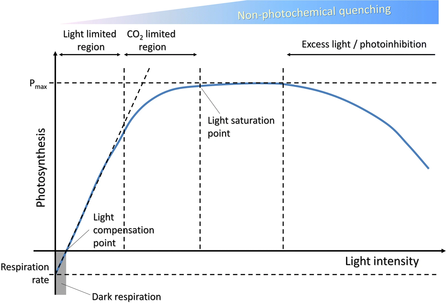
There are many examples of correlations that are not causal (also called spurious correlations), for example those collected by Tyler Vigen. Perhaps counter intuitively, there are also clear cases where a causal relationship does not lead to a correlation (See Figure 6.3 for an example in the plant sciences).
A strong scientific argument based on correlation builds on a few principles, which are outlined here. Building scientific arguments in general is a fundamental aspect of good science, but outside of the scope of this course.
When describing correlations, consider the following:
Take home message: A correlation coefficient is evidence, not a verdict. Strong scientific arguments combine visual inspection, use appropriate methods, consider effect size, and include (biological) reasoning about the context.
Exercise 6.9 Revisit Exercise 6.7: Are there any groups of variables that are all correlated to eachother? How would you interpret such a group of variables? Which of the steps of Tip 6.1 can you apply, and which are not feasible? How does this affect your conclusions?