# Executing this code in RStudio mimics how Quarto parses code and should produce the same error.
code <- "
# Syntax error example 1, missing closing bracket
collection <- c(1,2,3,
"
parse(text = code)5 Debugging and testing
Programming and scripting for data analysis is not only about writing code that runs. It is perhaps even more important to write code that produces correct and interpretable results.
Errors in code can become especially dangerous when they silently produce wrong results without throwing errors. In this chapter we will go over different types of errors and warnings and how you can solve and prevent them.
Warning 5.1: Data analysis code gone wrong, famous examples
In the late 2000s, researchers claimed that gene-expression data from cancer cell lines could be used to predict which chemotherapy drugs would work for individual patients. These results were considered so promising that human clinical trials were started based on the predictions. Later, independent scientists tried to reproduce the analysis and found that the problem was not the biological question or the statistical methodology, but simple bugs in the data-analysis code1. Gene-expression tables had been misaligned with patient labels, some samples had been accidentally swapped, and categorical variables had been silently reordered by the software. Because the analysis pipeline contained no checks that data and labels still matched, these errors went unnoticed. The models therefore looked highly accurate, while in reality they were making predictions close to random guessing. When the mistakes were corrected, the supposed drug-response signatures disappeared. Several papers were withdrawn and the clinical trials were stopped. This episode is now a classic warning that small programming errors can lead to large scientific and real-world consequences. The take home message: careful debugging and reproducible workflows matter in data-driven biology.
We will work on two complementary skill sets:
- Debugging and error handling: what to do when your code (or someone else’s code!) does not work as intended.
- Testing and validating: how to formally verify your code works as intended
5.1 Debugging and error handling
Bugs and errors go hand in hand: a bug is an error or flaw in a program that causes it to behave differently from what the programmer intended. Bugs can cause code to crash with an error, produce warnings, or even run without complaint while giving incorrect results.
Bugs arise for many reasons: misunderstandings about how a function works, incorrect assumptions about the data, edge cases that were not considered, or simple typing mistakes. Importantly, a program can be syntactically correct (it runs) and still contain bugs if the logic is wrong.
Debugging is the process of identifying, understanding, and fixing these bugs. Rather than trial-and-error, effective debugging relies on systematically inspecting code, checking assumptions, and narrowing down where the program’s behavior diverges from expectations.
NoteAbout the term “bug”
The word “bug” to describe a programming error is often linked to Grace Hopper. In 1947, while working on the Harvard Mark II computer, her team found that a malfunction was caused by a real moth trapped in a relay (back then computers where large devices that filled entire rooms). The insect was taped into the logbook with the note “First actual case of bug being found”.
Although the term bug was already used informally in engineering, this incident popularized it in computing. It nicely illustrates an important idea: bugs can arise from unexpected causes, and finding them requires careful investigation rather than guesswork.
Tip 5.1: How to debug
The main approach to debugging (potentially complex) code is to be systematic. The following steps help in identifying the underlying problem:
- Reproduce the issue: make sure you consistently see the bug. Does it only occur on a specific dataset? Or under other specific conditions? These can provide hints.
- Isolate the problem: (especially when working with larger functions or big datasets) Narrow down where the error actually comes from. Adding print statements or commenting out specific sections can help. Switching to a small test dataset can be useful too.
- Understand/hypothesize: once you figured out where the error occurs, check what you expected to happen and verify this is (or is not) happening.
- Fix and verify: Implement the fix, then test the code by reproducing the original conditions under which the error occurred.
To better understand what can cause your code to misbehave, it is important to understand a little bit about different types of errors in R. The following section covers syntax errors, runtime errors, warnings, and logical errors.
Syntax errors
These errors often pop up when you are in the process of writing some new code. Simply put, a syntax error is any form of mistake where your code does not follow the syntax definitions of the R language. As a consequence, the code cannot be parsed and executed by the interpreter. These error are caught relatively easy, because any syntax error will break the execution of your code. In addition, when viewing the full Quarto error message (see Note 5.1), a syntax error always starts with Error in parse(text = input): [...] indicating that parsing of the code failed.
Note 5.1: Rstudio VS Quarto syntax errors
The syntax errors you see in RStudio will look slightly different from what you see in this book (see Figure 5.1). This has to do with a difference between how RStudio and Quarto (used to create this book) read R code: RStudio reads line by line, Quarto reads an entire chunk. A scenario where this becomes relevant is when you try to render a notebook that contains a syntax error: then you will see the Quarto error, and not the RStudio error.
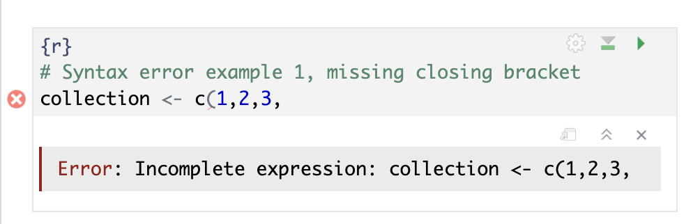
Replicating the Quarto error message in RStudio is possible, but requires some trickery: we force RStudio to read an entire chunk at once.
# Syntax error example 1, missing closing bracket
collection <- c(1,2,3,
Error in parse(text = input): <text>:3:0: unexpected end of input
1: # Syntax error example 1, missing closing bracket
2: collection <- c(1,2,3,
^Note that in R, code is interpreted and potentially executed on a line-by-line basis. Executing syntax error example 2 (below) in a clean environment will crash on the second line, but the first line will already have executed when the crash happens. As a result, in this example the variable collection will exist when the crash happens.
# Syntax error example 2, the last line is missing the closing bracket
collection <- c(1,2,3)
collection[1
Error in parse(text = input): <text>:4:0: unexpected end of input
2: collection <- c(1,2,3)
3: collection[1
^An exception to the line-by-line interpretation and execution is how code blocks are treated. Examples 3 and 4 show examples of syntax errors in code blocks: function definitions and loops are first completely interpreted before they are executed.
# Syntax error example 3, using incorrect bracket types
my_function <- function(arg){
  return(arg + 1)
]
Error in parse(text = input): <text>:4:1: unexpected ']'
3: return(arg + 1)
4: ]
^# Syntax error example 4, a syntax error in a loop
for (i in 1:3){
print(i)
print('There is a syntax error on this line)
}Error in parse(text = input): <text>:4:9: unexpected INCOMPLETE_STRING
4: print('There is a syntax error on this line)
5: }
^Runtime errors
A class of errors that will also break execution of your code are the runtime errors. Unlike syntax errors, the code can be parsed and interpreted, but there is an underlying problem when trying to execute the code that causes the interpreter to crash.
# Runtime error example 1: mismatched types
1 + "2"
Error in 1 + "2": non-numeric argument to binary operator# Runtime error example 2: trailing commas/empty arguments are valid syntax but can break at runtime
collection <- c(1,2,3,)Error in c(1, 2, 3, ): argument 4 is emptyRuntime errors are defined in code and make your code crash when some checks are failing. It is relatively straightforward to implement a check and produce an error (see runtime example 3 below). We will use this more strategically in Section 5.2.
# Runtime error example 3: implementing a custom check and producing a runtime error
my_function <- function(arg){
  if (arg > 3) {
    stop("arg must be <= 3, got ", arg)
  }
  print(arg)
}
my_function(2)
[1] 2my_function(4)Error in my_function(4): arg must be <= 3, got 4Warnings
In some cases, functions that you use might warn you when you are asking for unexpected behavior. One example we previously encountered are the warning messages of functions being overwritten when loading the tidyverse package. Warnings do not terminate your code, so just like logical errors you still get results. Unlike logical errors, you get some indication that there might be something not going as intended. Sometimes warnings can be safely ignored, sometimes they mean something is critically wrong.
# Warning example 1: converting strings to number raises a warning, but you still get a result
as.numeric(corre_continuous$species[1:5])
Warning: NAs introduced by coercion[1] NA NA NA NA NAExercise 5.1 In the example above (when attempting to convert a character to a number), do you think it is appropriate to raise a warning, or would an error be a better choice?
Implementing warnings in your own functions can be a very powerful tool to keep track of what is happening in your analysis (see example below).
# Warning example 2: raising a warning in a function

f <- function(arg){
  if (arg < 3) warning('arg must be >= 3, got ', arg)
  arg ** 2
}

f(2)
Warning in f(2): arg must be >= 3, got 2[1] 4It is important to realize that warnings, just like runtime errors (Section 5.1.2), are implemented in R code by e.g. package maintainers. This means that whether or not a function raises a warning when something unexpected happens always depends on the function, and whether the function author implemented a check or not.
Logical errors
In sections Section 5.1.2 and Section 5.1.3 we have covered what happens when e.g. a package maintainer implements a check in their code. But what about errors in your code that do not cause an error or raise a warning? These errors are potentially the most dangerous, because they do not show any direct visual clues that something is wrong. Any behavior of your code that does not result in the desired/expected result can be seen as a logical error. This can range from explicit mistakes in an implementation (e.g. messing up a mathematical calculation), to not realizing some hidden behavior of a certain function, to simple typo’s in variable names. The example at the start of the chapter (Warning 5.1) is an example of logical errors: the code ran to completion and produced results, but due to some mistakes in the implementation the results were incorrect.
The crucial problem here is that there is nothing in the code that checks assumptions or e.g. enforces certain properties of datasets/results. In Exercise 5.3 and Section 5.2 we explore in more detail how you can implement some of these checks yourself.
Exercise 5.2 (Identify the error) For each of the following 10 exercises, identify the type of error, and fix the code so that it works as expected. The aim of this exercise is to develop some intuition, so first try to do this without executing the code!
# Exercise 1: Calculating average leaf Nitrogen content
mean(corre_continuous$leaf_N

# Exercise 2: Finding the most common growth form
mean(corre_categorical$growth_form)

# Exercise 3: Is there a relationship between plant family and leaf N content?
cor.test(corre_continuous$family, corre_continuous$leaf_N)

# Excercise 4: What is the average leaf dry mass?
mean(corre_continuous$leaf_dry_mass, na.rm = TRUE)

# Exercise 5: Select all the entries for the grass family
subset(corre_continuous, family = 'Poaceae')

# Exercise 6: Calculate mean leaf are
mean(corre_continuous$SLA)

# Exercise 7: Select the leaf area for the 1,000th plant
corre_continuous$leaf_area[10000]

# Exercise 8: Compute the average seed dry mass for grasses
subset(corre_continuous, family == 'Poaceae')$seed_dry_mass |> mean(na.rm = TRUE)

# Exercise 9: Compute the mean SLA for a specific family
mean_trait_by_family <- function(dataset, trait){
  mean(dataset[[trait]], na.rm = TRUE)
}
mean_trait_by_family(corre_continuous, 'SLA')

# Exercise 10: log-transform seed dry mass
log(corre_continuous$seed_dry_mass)
Exercise 5.3 (Upgrading the implementation of the variance calculation) In Exercise 4.4 you implemented the calculation of the variance. Here, you will make that function a bit safer to use. Add the following checks, decide yourself whether it should be a warning or an error:
- The variance of zero or one numbers is undefined
- The variance of a collection of all the same numbers (e.g.
c(4,4,4)) is zero
Hints:
You can implement a check with
ifandelse:if (condition) { # Code to run when condition is TRUE } else { # Code to run when condition is FALSE }In this case
conditionmust evaluate toTRUEorFALSE, e.g.is.numeric(column)orlength(input) == 3. You don’t always need theelsepart.You can throw an error with the
stop()function.You can raise a warning with the
warning()function.
5.2 Testing and validating
In Section 4.1 we discussed how and when to use functions. It turns out that by following our rule of thumb for when to create a function1 we create functions that are often straightforward to test. In Section 5.2.1, we discuss what we mean with testing a function, and we highlight two ways of testing your code. In addition, we briefly discuss the difference between testing and validating in Section 5.2.2.
Testing code
As an example, we revisit Exercise 4.6: we want to compute the difference between the mean and the median many times, so it makes sense to implement this in a function.
# Example function that we are going to test
mean_median_difference <- function(input){
  # We compute the absolute difference so it doesn\'t matter which number is bigger
  abs(mean(input, na.rm = TRUE) - median(input, na.rm = TRUE))
}

mean_median_difference(grassland_traits_environment$ld)
[1] 0.0558324Our example function does not throw errors or raise warnings, and it produces a result, so far everything looks alright! But apart from just reading and checking the code, we don’t really know whether our function behaves as intended. This is where it becomes useful to implement some checks of our code, using code. In this book we limit ourselves to unit testing: the process of testing small isolated components (i.e. functions). Approaches for testing integrations or entire systems exist as well, but these are outside of the scope of this course.
The key component of testing functions is to identify a set of inputs for which the output is known. This often means coming up with small toy examples. In the case of our example function, the computations are relatively straightforward for small amounts of numbers, so we implement a simple testing procedure below:
# We will test our function on a small test dataset for which we know the expected outcome of our function
test_input <- c(1, 2, 2, 3, 7)

# The mean of this collection of numbers is 3, and the median is 2, so the difference should be 1
known_output <- 1

# We run out function on the test input to acquire the test output
test_output <- mean_median_difference(test_input)

# We check if the acquired output matches the expected output
if (test_output == known_output) {
  print('Great success!')
} else {
  stop(paste('Expected', known_output, 'but got', test_output))
}
[1] "Great success!"Exercise 5.4 (Experiment with the simple testing example) Create a few alternative testing datasets with known outputs, and use them with the simple testing code above. Also try out what happens when the known output does not match the test output.
A careful observer might already have identified that our simple testing procedure that we describe above always does the same steps for every test you would design. This makes it a very good candidate for extracting the logic into a function, which is exactly what the testthat package does! More precisely, the testthat package includes a lot of functionality for quickly and reproducibly writing unit tests, with functions that closely resemble the english language. This latter property makes for very readable testing code:
# We implement the same test as before, but now with the testthat package, and including more test cases
library(testthat)

test_that("Correct difference between mean and median is calculated", {
  expect_equal(mean_median_difference(c(1, 2, 2, 3, 7)), 1)
  expect_equal(mean_median_difference(c(1, 2, 3)), 0)
})
Test passed with 2 successes 🥇.In addition to testing expected outputs, the testthat package makes it very easy to test other behavior of functions as well, for example whether it correctly produces an error when incorrect input data is provided:
library(testthat)

test_that("Error is thrown on incorrect input", {
  expect_error(mean_median_difference('String'))
})
── Warning: Error is thrown on incorrect input ─────────────────────────────────
argument is not numeric or logical: returning NA
Backtrace:
▆
1. ├─testthat::expect_error(mean_median_difference("String"))
2. │ └─testthat:::quasi_capture(...)
3. │ ├─testthat (local) .capture(...)
4. │ │ └─base::withCallingHandlers(...)
5. │ └─rlang::eval_bare(quo_get_expr(.quo), quo_get_env(.quo))
6. └─global mean_median_difference("String")
7. ├─base::mean(input, na.rm = TRUE)
8. └─base::mean.default(input, na.rm = TRUE)
Test passed with 1 success 🌈.Note that whereas we are incorrectly using the mean_median_difference() function and so it raises an error, this is actually part of the test, and so the test itself is successful.
In summary: unit testing describes a set of tests that are automated in code. Tests are designed to throw an error upon unwanted behavior of the code, so if all tests pass this is a good sign of properly working code.
Exercise 5.5 Note that the error test in the example above raises a warning? Can you find out where this warning is coming from and what is causing it? Hint: recall Tip 5.1. Why does the test still pass if a warning is raised? What would be the best way to get rid of this warning: adding additional tests, or changing the function?
Exercise 5.6 In Exercise 5.3 you implemented some warnings and errors for your code that calculates the variance. Write tests with the testthat package to verify the calculation, errors, and warnings of your function.
Validating code
In the previous section we looked at formally verifying the correctness of a piece of code. In other words, we answered the question “Does the code do what we programmed it to do?”. This an important aspect of producing reliable analysis results, but is not the only thing that matters. In addition to formal correctness, you should also always think about whether it makes sense what your code is doing. In this course, we call this validating: “Is the code solving the right problem?”.
For validation, we typically do not use automated procedures. Rather, we rely on external comparisons: this can be checking plausability of results with literature, but also submitting your code to expert- or peer review (This is in part why we do weekly code review sessions!).
Ultimately, you want your code to be both tested and validated (see Table 5.1), but it takes some time and effort before you get there!
| Tested | Untested | |
|---|---|---|
| Validated | Provably correct, relevant results | Correct idea, buggy execution |
| Unvalidated | Bug-free implementation of a flawed idea | Don’t go here 💀 |
Exercise 5.7 Revisit Warning 5.1 and decide whether testing, validating, or both went wrong. How should plant scientists make sure they do better than this example?