4  Functions and summary statistics

In this chapter we expand on two concepts that we encountered in the previous week: functions, and summarizing a dataset with numbers. We start with a few concepts on what functions are and when to use them in Section 4.1, and we apply these concepts in Section 4.2 to implement the calculation of some useful dataset summaries. We will explore several numerical summary techniques, such as computing the mean and standard deviation of a numeric variable, or counts/frequencies of a categorical variable. We finish the chapter with a brief section on various other programming concepts that you typically encounter when doing exploratory data analysis (Section 4.3).

Exercise 4.1 (Inspecting the datasets for this week) Make sure you have installed the PlantEDA data package (see Note 1). Inspect the documentation for the three datasets: corre_continuous, corre_categorical, and grassland_traits_environment. Where do these datasets come from? What is the difference between the three datasets? In what type of object are these datasets stored?

library(planteda)

# Loading and inspecting the corre_continuous dataset
data('corre_continuous')
?corre_continuous

4.1 Functions

In the previous chapters we have encountered functions. So far, we have used these functions to our advantage, but we have mostly glossed over what a function is, and when it is most appropriate to use functions. In this section we go into a bit more depth to highlight the most important practical aspects of functions in R, whilst avoiding unnecessary theoretical detail as much as possible.

What is a function?

A function can be concisely described as a reusable piece of code that takes input values (arguments), performs an operation, and returns a result. Some clear examples of this are the functions you have used from some of the packages you used (e.g. the read.csv() or ggplot() functions). It is important to make the distinction between the function definition, which is the piece of code that describes what the function does, and calling a function, which is where the code is used (See Note 4.1).

Note 4.1: R function syntax

Function definition

Named functions in R are all functions that are assigned a variable name (see example below).

# Named function example  
1function_name <- function(argument){
2  # function body
3  return(...)
4}

1

First line of a function definition, in this case the function is assigned to a variable named function_name. { indicates the opening of the function body.

2

The function ‘body’ contains all the logic that will be executed upon function execution

3

The return statement provides the result of the computation performed inside the function

4

The function body is closed with }

Not all functions have to be assigned to variables: anonymous functions are inline function definitions that are not assigned to a variable. As such, they can not be executed anywhere else. A clear use case of anonymous functions is in e.g. the apply approaches where a simple operation is applied to multiple elements of a collection (see example below).

# Anonymous function example
1sapply(
2  1:3,
3  function(element){
    # apply operation on element (in this case a number in the range 1 to 3)
    return(result)
  }
)

1

sapply applies a function to a collection. The first argument to sapply is the collection, the second argument is the function that will be applied.

2

In this example we apply our function to the range 1:3

3

Anonymous function: in this sapply example, it will be applied to the range 1:3. The function will receive as argument one element from the collection, so in this case a single number.

For short, easy to understand operations, the one-line function syntax is sometimes used.

# one-line named function
1function_name <- function(arg1, arg2) arg1 + arg2

1

A one-line function definition can omit the curly braces ({ }).

Using (executing/invoking/calling) a function

A function is executed by using the parenthesis (( )) syntax.

# Executing a previously defined function
function_name(arg1, arg2)

Getting help for existing functions

Base R functions and functions that are imported from packages come with documentation on what the function does, and how to use them. This documentation typically includes a description of all the possible arguments for a function, and a few examples. The documentation for a function can be invoked by prefixing the function name with a question mark (?) in the R console.

# Typing this in the console will open the documentation for the function (if it exists)
?function_name

In addition, executing the function name in the R console (without parentheses!) prints the function definition.

# Typing this in the R console will print the function definition
function_name

Exercise 4.2 (Inspect some function definitions and documentation) To get familiar with inspecting function documentation and definition, execute the following commands and note down what you find:

• ?read.csv and read.csv
• ?mean and mean
• ?filter and filter

Why (and when) use a function?

As you become more experienced and proficient in performing data analysis in R, you’ll find that the amount of code you write to do these analyses expands. The basic steps of a data analysis pipeline (loading, inspecting, cleaning, analyzing, presenting, see Tip 1) will often be repeated multiple times. These are very good cases of where defining a function makes sense! By bundling a sequence of operations into a function, your code improves in three key ways:

1. Clarity: instead of a long list of R commands, readers can read more ‘high-level’ code and more easily understand the main steps being performed
2. Re-usability: write the analysis logic once, and reuse it across different datasets without copying and pasting. (Packages are the ultimate example here).
3. Maintainability: If something changes in your workflow, updating the logic in one place (i.e. at the function) makes sure all places where the logic is applied are also updated.

A few typical situations where it thus makes sense to implement a function: you’re copying and pasting the same code over and over again; a sequence of steps represent a logical subtask; applying the same steps to different variables or datasets. In addition, functions make your code easier to document and test (more details on testing will be discussed in Chapter 5).

Tip 4.1: Naming functions (is hard)

Should my code be a function? A straightforward way to determine whether a piece of code can be extracted into a function, is how easy it is to give a name to the collection of steps being performed. You’ll be surprised how hard it can be to give intuitive names to functions! In fact, there are entire books written about just this.

Base R has some good examples (both good and bad):

• read.csv() does what it says: it reads a csv file. The name matches perfectly with what the function does.
• apply() is much less straightforward: the name does not tell you what is being applied, or what it is being applied to. You need to read the documentation carefully to figure out these things, and how to actually use this function.

Exercise 4.3 (Revisite some code from last week) Let’s take a look at some code from last week:

1. Compare the code for Exercise 1.11 and Exercise 1.12. Which parts are shared? What would the function for doing the shared parts be called?
2. Revisit the code for Exercise 1.12. There are a few steps in the for loop that perform (more or less) isolated tasks. Could you come up with logical names for these steps? Do you think it makes sense to extract these steps into individual functions?

4.2 Summary statistics

To explore new and previously unseen datasets, we tend to follow the data science cycle (Tip 1). Summary statistics play a key role in both the inspect and analyse parts of this cycle. A summary statistic is something that is easy to calculate, and gives you some insights into what the data in your dataset looks like. By calculating a few different summary statistics, you can get a quick overview of a dataset, and potentially diagnose some easy to spot issues.

In this section, we present the main summary statistics that you will use for summarizing a new dataset. For most summary statistics, we perform some arithmetic and computation. This gives us an excellent opportunity to implement what was covered in the previous section on functions!

Mean

Perhaps one of the simplest and most intuitive summary statistics is the mean (typically indicated with the greek letter \(\mu\)). The mean can be calculated as the sum of all values in a variable divided by the number of values in that variable (Equation 4.1).

\[ Mean(X) = \mu = \frac{1}{N}\sum_{i=1}^{n}{x_i} \tag{4.1}\]

The simplest and most direct interpretation of the mean is that it represents the average value of a variable. A slightly more statistically oriented interpretation is that the mean represents the expected value. In other words: if you have no other information, the mean would be your best guess¹ on average. In the example below this would mean that your best guess of the leaf dry matter content of a plant, without knowing anything else about that plant, would be 0.25\(g/g\) (The blue solid line in Figure 4.1).

Being a statistical programming language, R comes with a default function to calculate the mean:

# Calculate the average leaf dry matter content
mean(corre_continuous$LDMC)

[1] 0.2535559

Note 4.2: Example: implementing the mean calculation in a custom function

Since R already comes with a default function to calculate the mean this example might seem redundant. At the same time, this gives us the opportunity to check whether our custom implementation returns the correct result.

# Here we define a function to perform the calculation of the mean, 
# closely following the mathematical description
custom_mean <- function(input){
  total = sum(input)
  number = length(input)
  return(total / number)
}

# This should give the same result as using the default `mean` from R
custom_mean(corre_continuous$LDMC)

[1] 0.2535559

Variance

Where the mean describes the average value of a variable, the variance describes how much individual data points differ from the mean. More precisely, the variance is defined as the average of the squared differences between each observation and the mean (Equation 4.2). In other words: for each value we compute how far it is from the mean, square this difference, and then average these squared deviations. In our example on leaf dry matter content, the variance quantifies how much individual plant species differ from the average leaf dry matter content. Note that squaring the difference has two important consequences: positive and negative differences contribute equally, and large differences contribute relatively more than small differences. A consequence of this last property is that the variance is relatively sensitive to outliers in the data.

\[ Variance(X) = \sigma^2 = \frac{1}{N}\sum_{i=1}^{n}{(\mu-x_i)^2} \tag{4.2}\]

Standard deviation

One slight downside in interpreting the variance is that the units are squared compared to the data points. In our example, leaf dry matter content is measured in \([g/g]\), and as a consequence the mean is also in \([g/g]\). However, the variance is in \([(g/g)^2]\), which makes interpretation less straightforward. A common and useful solution is to take the square root of the variance, which results in the standard deviation (See Equation 4.3 and the striped blue lines in Figure 4.1).

\[ StandardDeviation(X) = \sigma = \sqrt{\frac{1}{N}\sum_{i=1}^{n}{(\mu-x_i)^2}} \tag{4.3}\]

Exercise 4.4 (Implement the variance calculation in a custom function) Just like in the previous example on the mean, R has a built-in function to calculate the variance (var). To practice implementing custom functions, in this exercise you will implement the calculation of the variance yourself. Compare the output of your custom function to the output of the built-in var function to check your work.

# Implement the calculation of the variance in a custom function
custom_variance <- function(input){
  # ... some initial calculation goes here
  variance <- # ... final calculation goes here
  return(variance)
}

Median

The mean and variance summarize the data by combining all values using arithmetic operations. In contrast, some summary statistics depend only on the relative order of the values, not on how large or small individual observations are. These order-based statistics often behave more robustly when extreme values are present (in other words: they are less sensitive to outliers). In the following section we discuss the median (the striped blue line in Figure 4.1), its generalization into quantiles, and the accompanying interquartile range (the dotted blue lines in Figure 4.1).

The simplest and most direct interpretation of the median is that it represents the middle value of a variable. More precisely, the median is the value that splits the data into two equally sized parts when the observations are sorted. In other words: half of the observations are smaller than the median, and half are larger. In the example below this would mean that half of the plants have a leaf dry matter content below the median value of 0.24\(g/g\), and half above.

# Calculate the median leaf dry matter content
median(corre_continuous$LDMC)

[1] 0.2397274

Exercise 4.5 (Interpret the mean and median) When computing the mean and median of the leaf dry matter content, we observe a (small) difference. How do you interpret this difference? (You can use Figure 4.1 for visual intuition).

Exercise 4.6 (Summarize the corre_continous dataset) Write some R code to calculate the difference between the mean and the median of all continuous variables in the corre_continuous dataset.

Tips:

• The function colnames() returns the names of all columns in a dataframe
• You can loop over colnames
• You can access an individual column of a dataframe by name and using double square brackets –> dataframe[[colname]]
• You can check whether something is numeric with the is.numeric() function

Quantiles

Quantiles generalize the idea of the median by describing values at fixed positions in the sorted data. A \(q\)-quantile is the value below which a fraction \(q\) of the observations fall. In other words: a \(q\)-quantile splits the data into a lower part containing a fraction \(q\) of the observations and an upper part containing the remaining fraction. For example, the 0.25-quantile (also called the first quartile) is the value below which 25% of the data lie.

Exercise 4.7 (Implement quantile calculation in a custom function) In this assignment you will implement the calculation of quantiles for a continuous variable. Once again, you can check your implementation by comparing to the built-in quantile function. Unlike the mean, calculating quantiles is not just a sequence of arithmetic. To help you get started, here are some pointers:

• The number of elements in a collection can be calculated with length
• A collection can be sorted with sort
• Numbers can be rounded with round, the resulting integer can be used as an index

custom_quantile <- function(data, quantile_percentage){
  # Do stuff here
  quant <- # Some more calculations
  return(quant)
}

Interquartile Range (IQR)

A commonly used measure of spread in the data based on quantiles is the interquartile range (IQR). The IQR is defined as the difference between the third quartile and the first quartile. In other words: it measures how much the middle 50% of the data vary. In the example below this would quantify the spread of leaf dry matter content values for the central half of the plants (also see the dotted green lines in Figure 4.1).

# Calculate the middle 50% of values (AKA the interquartile range IQR) for leaf dry matter content
IQR(corre_continuous$LDMC)

[1] 0.1105531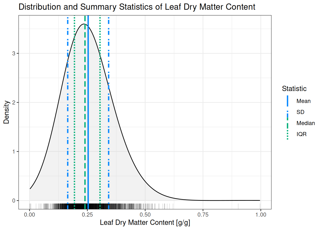

Figure 4.1: A visualization of various summary statistics computed on the Leaf Dry Matter Content variable in the CoRRE dataset. Blue lines represent the mean and standard deviation, green lines represent the median and the interquartile range. Individual datapoints are indicated on the X axis. The effect of a few large values can be observed in the difference between the mean and the median.

Exercise 4.8 (Creating and interpreting a boxplot) Create a boxplot for leaf dry matter content using the corre_continuous dataset and compare to Figure 4.1. Which summary statistics do you recognize? (You can use either base R boxplot or ggplot with the geom_boxplot geom.)

Counts/proportions

All the summary statistics we have discussed so far apply to numeric variables. Of course, not all data is numeric: one commonly encountered type of data is categorical. The most commonly used technique to summarize categorical data is to count the number of elements in each category, and potentially convert these counts into proportions. In the example below we use the built-in table and proportions functions to calculate counts and proportions respectively for how many species are known to be clonal.

# Counting how many plant species are clonal
table(corre_categorical$clonal)

       no uncertain       yes 
     1646       442      1991 

# Calculating the proportions of how many plant species are clonal
proportions(table(corre_categorical$clonal))

       no uncertain       yes 
0.4035303 0.1083599 0.4881098 

Putting it all together

Throughout this chapter, we introduced summary statistics by first focusing on their individual roles and functions—such as mean() for central tendency, sd() and var() for spread, median() and quantile() for robustness against outliers, and counting functions for categorical data. While these functions are useful when you want a specific numerical result, R also provides a convenient way to combine several of these descriptive measures in a single step using the function summary(). For numeric data, summary() computes the minimum, first quartile, median, mean, third quartile, and maximum, bringing together measures of location and spread that you have already seen separately in this chapter. For categorical variables, the same function switches behaviour and returns counts per category, which mirrors the tabulation-based summaries discussed earlier. As such, summary() acts as a compact overview function: it does not replace the individual summary statistics, but it provides a quick first impression of the data using a consistent and easy-to-interpret output.

Exercise 4.9 (Putting all summary statistics into a single overview) Use the summary() function on both the corre_categorical and corre_continuous datasets. Describe your findings, making note of the following things: (1) what are the data types of the different variables? (2) How many NAs are there in the dataset? (3) Are there any variables with extreme values?

NoteA note on hypothesis testing

In this chapter, we describe summary statistics mostly in the context of the inspect step of the data science cycle (Tip 1). However, some of these summary statistics also appear in the analyse step! In that context, some of these statistics are used in e.g. statistical hypothesis testing. A clear example is the t-test (Equation 4.4), which uses the means and standard deviations to compute a p-value for a observed difference. The exact formulations of the statistical tests belong in a statistics course, and are outside of the scope of this book. However, here we show a formulation of the t-test as an example, and to highlight the appearance of the mean and standard deviation. Note: here we use \(\bar{x}\) and \(s\) for the mean and standard deviation respectively. The symbols \(\mu\) and \(\sigma\) are typically used in formulas and theory but refer to ideal quantities rather than observations of a dataset (which would be part of a follow-up statistics course!). \[ t = \frac{\bar{x}_1 - \bar{x}_2}{\sqrt{\frac{s_1^2}{n_1}+\frac{s_2^2}{n_2}}} \tag{4.4}\]

4.3 Other programming techniques

In Section 4.1 we have discussed the basics of functions in R. In your data analysis practice, this will be the most useful tool that you use to make your code readable, reusable, and maintainable. However, when working with R a bit more (and perhaps also using other programming languages), you likely encounter some other programming techniques as well. In this section we briefly highlight a few common programming techniques to raise awareness, but we do not go into full detail on how these techniques work.

TipAdvanced R

The book Advanced R¹ provides a good and detailed overview of some of the topics in this section. It’s not very beginner friendly though!

Object Oriented Programming (OOP)

In addition to functions, R also supports object-oriented programming (OOP). In OOP, data and the operations that act on that data are conceptually bundled together into objects.

In practice, you have already been using OOP in R, even if you were not aware of it. For example, when you call summary() on different types of objects, R automatically chooses an appropriate method depending on the object:

# These all provide useful summaries, but are implemented completely differently under the hood
summary(my_numeric_vector)
summary(my_data_frame)
summary(my_statistical_model)

Although the function name is the same, the behavior differs. This is an example of method dispatch, where R selects the correct method based on the class of the object.

For most data analysis workflows, it is not necessary to write your own object-oriented code. However, understanding that many R functions behave differently depending on object class helps explain why the same function call can produce different results in different contexts.

Scoping rules

The scope of your code determines where R looks for objects such as variables and functions.

When a function is executed, R first looks for variables inside the function itself. If a variable is not found there, R then searches in the surrounding environments. This behavior is known as lexical scoping.

# Scoping example: var1 is defined in the outside scope
var1 <- 10

# This example function takes no arguments
f <- function() {
  # var2 is defined in the function scope
  var2 <- 5
  # We still have access to the outside scope
  return(var1 + var2)
}

# Executing the function performs the calculation. Note there are no arguments provided!
f()

[1] 15

Exercise 4.10 (Thinking about scope) In the example above var1 and var2 are available in the function scope (Verify how you know this is true!). Is var2 available outside of the scope of the function (e.g. what happens if you try to print var2 outside of the function?)

Vectorization

Many quantitative operations and functions in R are vectorized. This means that the semantics of the operation are applied to a collection of elements individually, without having to write additional loops or other code

# Vectorization example, the square root is calculated for each number individually
numbers <- c(25, 9, 5)
sqrt(numbers)

[1] 5.000000 3.000000 2.236068

There is no single diagnostic for determining whether a function is vectorized or not. Often the semantics of the function will give a hint: if the operation should work on multiple elements, and the number of return values is the same as the number of inputs, a function is a good candidate for being vectorized. Some examples: most arithmetic is vectorized, read.csv() is typically not expected to work on a collection of filenames (so not vectorized), and mean() summarizes multiple numbers into a single statistic (also not vectorized).

Exercise 4.11 (Vectorization alternatives) What other language constructs have you already encountered that perform the same function as vectorization? (Hint: look back at Exercise 1.11)

1.

Wickham, H. Advanced R. (Chapman; Hall/CRC, 2019). doi:10.1201/9781351201315.

---

1. “Best guess” is kept informal here. A full probabilistic treatment exists, but is beyond the scope of this book