📘 This content is part of version: v1.0.0 (Major release)In this chapter you will learn about various high-throughput biomolecular measurement techniques.
This chapter discusses what we call omics measurements: genomics, transcriptomics (gene expression), proteomics and metabolomics. Omics technologies measure the presence, levels and/or interactions of different types of molecules in the cell, obtaining data for all molecules at once (see Figure 1). Genomics focuses on the entirety of information that can be derived from genomes (structure, function, evolution, etc.). Transcriptomics, proteomics, and metabolomics focus on gene expression, protein, and metabolite levels, respectively. Finally, phenomics measures the outward appearance and behavior of cells and organisms.
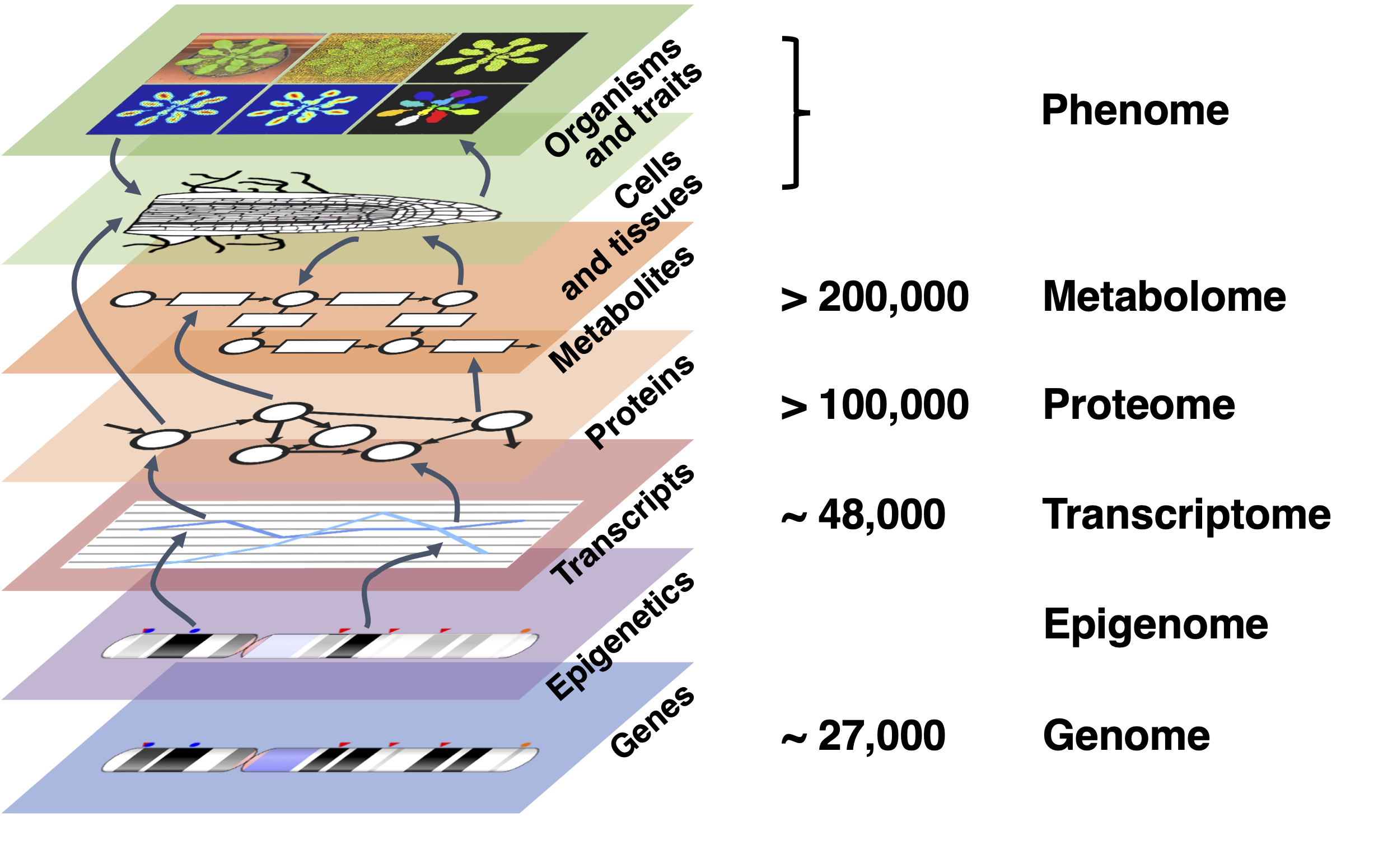
Figure 1:Different -ome levels, here illustrated with estimated numbers for Arabidopsis thaliana. Genes are expressed as transcripts, under the influence of epigenetic regulation. Transcripts are translated to proteins, that perform a myriad of functions in the cell, among which the enzymatic regulation of metabolic reactions that consume and produce compounds. Proteins and metabolites regulate interactions between cells involved in growth and development of tissues, finally leading to organisms and observable traits. At each level, there are now means to measure molecule presence/absence, levels and certain types of interactions at a very broad, so-called “genome-wide” scale. Credits: CC BY-NC 4.0 Ridder et al. (2024).
The concept of genes is central to the dogma of molecular biology; it therefore makes sense that much early research was invested in sequencing genomes. These genomes were then annotated for genes, with accompanying predicted protein sequences. This focus on sequences has dominated much of the first decades of bioinformatics, leading to the development of the databases and tools for sequence alignment, phylogeny and sequence-based prediction of structure that were discussed in earlier chapters. However, after sequencing the first genomes it became clear that the DNA tells only part of the entire story: the expression of genes and proteins and their interactions in processes within and between cells govern how cells and organisms behave. This led to research in functional genomics and systems biology, for which computational data analysis of other omics level data have become indispensable.
Below, genomics will first be introduced, along with the most relevant technology: sequencing, which is also used for transcriptomics. This will be followed by an introduction to functional genomics and systems biology and brief overviews of transcriptomics, proteomics, metabolomics, and phenomics, as well as the main types of data analysis involved.
Genomics and sequencing
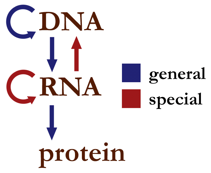
Figure 2:Information flow in the cell. Credits: CC0 1.0 Narayanese (2008).
DNA is the starting point in the chain of biological information flow (central dogma). From DNA we progress through transcription and translation towards whole organisms and their phenotypes. So, it is fitting to start at the beginning. Even before people knew about DNA and its role as keeper of hereditary information, they were aware that parental characteristics are inherited by offspring. Around 1866, Gregor Mendel was the first to perform detailed experiments testing heritability. He first described ‘units of heredity’, later named genes. Today, we know that genes are encoded in the DNA in our cells. Our understanding of genes has expanded to a more complex concept, focused on stretches of DNA coding for proteins or RNA. The term genome was originally used to describe all genes in an organism or cell, but now refers to the full DNA content of a cell.
Genomes
The history of genome sequencing and the importance of the human genome project in the development of sequencing methods is described in Box 5.1. With the rapid development of sequencing technology, our understanding of genomes and their content has grown as well. We now know that genomes vary greatly in terms of size, chromosome numbers, and ploidy (Figure 4), as well as gene content (Table 1). Genome sizes range from 100kb in bacteria to more than 100Gb (Giga bases) in plants. Humans have a genome size of 3.2Gb.
Table 1:Genome size and number of genes of model species
| Species | Genome size (kb) | Number of genes | Number of transcript | Average gene density (kb) |
|---|---|---|---|---|
| E. coli | 4.6 | 4288 | 4688 | 1.1 |
| S. cerevisiae | 12.1 | 6600 | 7127 | 1.8 |
| C. elegans | 100 | 19985 | 60000 | 5 |
| D. melanogaster | 143.7 | 13986 | 41620 | 10.2 |
| A. taliana | 119.1 | 27562 | 54013 | 4.3 |
| H. sapiens | 3100 | 20077 | 58360 | 154.4 |
Not only the genome size varies greatly between organisms, in eukaryotes the number of chromosomes and chromosomal copies (ploidy) do too. Chromosome numbers range from 4 in fruit fly (Drosophila) to 23 in human to 50 in goldfish and 100+ in some ferns. Similarly, ploidy ranges from haploid (single set of chromosome(s), ploidy of N) and diploid (two copies, ploidy of 2N) to polyploid (more than 3 copies), with at the extreme end ferns with ploidy levels of over 100. Gene numbers also vary per species; at the low end, bacterial endosymbionts have 120+ genes, whereas most higher eukaryotes (including humans) have between 15,000 and 25,000 genes and some plants can have more than 40,000 genes – rice has over 46,000.
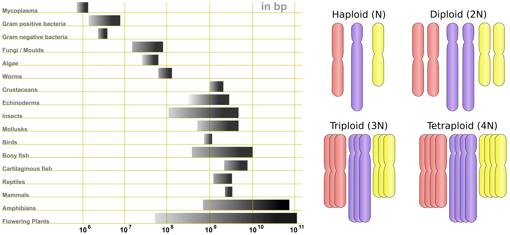
Figure 4:Left, variety of genome sizes. Credits: CC BY-SA 3.0 Abizar (2010); right, examples of ploidy. Credits: CC BY-SA 3.0 Ehamberg (2011).
Genome sequencing technologies
In order to study genomes, we need to have a human readable representation of them. This requires the ‘reading’ of the DNA molecules as A,C,T and Gs. This process of generating a genome starts with DNA sequencing, the detection of nucleotides and their order along a strand of DNA.
If you work with genome data, it is important to have a basic understanding of the technologies used and their strength and weaknesses.
This allows us to better understand the quality of the data we work with and what biological insights we can gain. For interested readers we provide a more detailed description of these technologies in a number of boxes at the end of this chapter.
Conceptually, there are three ways of sequencing:
Chemical sequencing relies on step-by-step cleaving off the last nucleotide from a chain and identifying it. Mainly due to the use of radioactive labels, this method was never widely used.
Sequencing-by-synthesis involves synthesizing a complementary strand base by base and detecting insertion at each position. This is currently the most widely used method, and various implementations are available. It is also referred to as Next-Generation Sequencing (NGS).
Direct sequencing involves directly measuring the order of nucleotides in a strand of DNA which is thus far only implemented in Oxford Nanopore sequencing.
Different technologies vary widely in the length of DNA sequences, called (sequencing) reads, they produce (the read length) and their throughput, which together determine the coverage: the (average) number of times each base in the genome is represented in a read. For some purposes, such as genome assembly, it is essential that this coverage is sufficiently high - depending on read length, between 50x to 100x. A number of sequencing devices and their capabilities in terms of read length and yield per run are shown in Figure 5.
Sequencing technologies also vary in the accuracy of base-calls (the detected nucleotide at a position). This accuracy is measured using quality or Q scores and they represent the probability that a base-call is incorrect. A higher Q-score is better. The most commonly used cut-off value is Q30 which corresponds to an incorrect base-call probability of 1 in 1000 and therefore an accuracy of 99.9%.
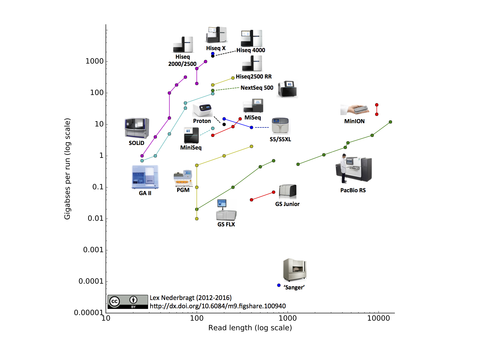
Figure 5:Sequencing technology, with yield per run vs. read length. Note the logarithmic scales. Multiple dots per technology indicate improvements in read length and/or yield due to upgrades. This figure is already outdated with higher yields produced by the Illumina NovaSeq and longer reads by both Oxford Nanopore MinION/PromethION and Pacbio Sequel II devices. Credits: CC BY 4.0 Nederbragt (2016).
Sanger sequencing
Sanger sequencing was the first ‘high-throughput’ method of DNA sequencing. For more details on its history and how it works, see Box 5.8.
In essence Sanger sequencing is a PCR reaction where step-by-step a copy of a DNA fragment is created using fluorescent nucleotides of different colors, the light of which is detected and translated to a nucleotide. Sanger sequencing needs many copies of a single, unique DNA fragment to be present in the sequencing reaction to ensure the light signal is strong enough to detect. The signal has to also be of a single color in each step, so the template sequences have to be all identical. This meant that in the sample preparation step fragments were cloned using either normal PCR or other large scale amplification methods. The requirement of uniqueness is the biggest drawback of Sanger sequencing.
Sanger sequencing was the main sequencing platform until around 2007. From 2004 onwards, it was increasingly superseded by what we call next-generation sequencing (NGS) methods. Today it is still used, among others to sequence PCR products to validate variants, to determine the orientation of genes in cloned vectors, or in microsatellite studies.
Next generation sequencing
Next-generation sequencing (NGS) technologies allow much higher throughput at far lower cost than Sanger sequencing, although it comes at a price: shorter reads and lower base-calling accuracy. These newer devices now produce billions of reads per sequencing run. Describing all of these methods in detail is beyond the scope of this course.
As with Sanger sequencing, NGS methods rely on amplification of a library of input DNA fragments to enhance the signal of the actual sequencing step. Most sequence data is nowadays generated by Illumina technology (or 3rd generation methods, see the next section) which allows for massive parallel sequencing of reads. How Sequencing-by-synthesis and Illumina patterned flow cells work is explained in detail in Box 5.9; below we list the main characteristics of the data.
Overall, Illumina reads are cheap, short and highly accurate.
3rd Generation sequencing
After the success of NGS, alternative so-called 3rd generation technologies were introduced to overcome some of the shortcomings, mainly the limited read length. All produce longer reads at lower yields, and generally have a slightly higher error rate than the methods described previously. They also perform what is called real-time sequencing: Each DNA fragment is sequenced completely in a continuous way, there is no need for individual cycles like in NGS.
PacBio
The most established method is PacBio single molecule real time (SMRT) sequencing. Compared to other methods it does not include a PCR step to amplify the signal of the template DNA. Instead, during the sequencing of an individual DNA molecule, light is emitted when a labelled nucleotide is inserted. This light is then amplified so that it can be detected. More detail can be found in Box 5.10.
Nanopore sequencing
The newest technology is nanopore sequencing, currently provided by Oxford Nanopore on the MinION and related devices (Figure 6). This technology is completely different to any of the others, in that it directly detects the order of nucleotides based on current changes caused by a single DNA strand being pulled through a protein nanopore embedded in a membrane (see Box 5.11 for more information). As with Pacbio sequencing read-length is determined by the length of the DNA template.

Figure 6:Oxford Nanopore MinION sequencer Credits: CC BY-SA 4.0 Ockerbloom (2020).
Quality control
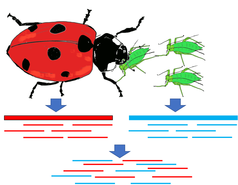
Figure 7:Causes for contaminated sequencing samples, using as example the ladybug and its main food source, aphids. Additionally all eukaryotes have a microbiome composed of prokaryotes, viruses, and small eukaryotes and these can also be present as contaminants. Credits: CC BY-NC 4.0 Ridder et al. (2024).
Before we can use the sequencing data for further analysis, we need to make sure the data is good enough.
A first step for quality control is to check the accuracy of the data. As sequencing technology is not perfect, errors will be present in the output. To minimize these, we remove poor quality reads or bases.
Errors related to sequencing itself are the result of base calling errors (substitution errors), uncalled bases (indels), GC bias, homopolymers, a drop of quality towards the 3’end of a read, and duplicates (amplification bias).
Sometimes what we sequence is correct, but not what we originally intended to sequence (Figure 7). Identifying contamination is important for genome assembly as we do not want to assign genome sequences to the wrong species. Imagine the confusion if the ladybug all of a sudden had genes for red aphid eyes. Tools exist to identify reads from contaminant species using sequence homology (e.g. blast).
In addition to contamination of the input sample, sequence data can also contain remnants of adapters and sequencing vectors, which can be removed with dedicated software.
It is important to assess the quality of the sequencing itself and the output data before further analysis.
Genome assembly
When no reference genome is available for a species, we need to assemble one, i.e. build one from scratch by putting together DNA sequence reads. Here we discuss the steps and considerations: First, we examine why we would want to create a reference assembly, and what types of references can be created. Next, the assembly process and its challenges are introduced. Finally, genome annotation and detection of structural variation are discussed.
Reference genome quality
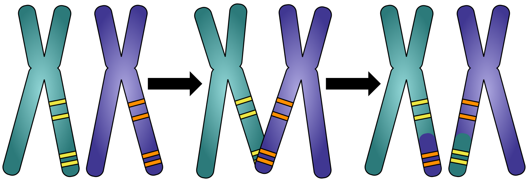
Figure 8:Co-segregation of alleles: Which parts of the genome were inherited together from either the mother or the father. Credits: CC BY-NC 4.0 Ridder et al. (2024).
Genomes can be reconstructed with different aims, which influence the required quality of the final assembly. The human genome, for example, has been assembled as far as possible and in 2021, the first telomere-to-telomere assembly was published, adding the final 5% of bases. It has taken enormous effort, both in terms of finance and labour, to get to this stage. This is neither feasible nor strictly necessary for each genome assembly project. Hence, most genome assemblies currently available are so-called draft assemblies, and most fully completed genomes are from bacteria and other species with small genomes. In terms of the assembly process, for eukaryotic genomes the euchromatic regions assemble best. Fortunately, these regions contain most of the genes, making draft assemblies useful for studying mutations or expression patterns. When we want to study larger features of the genome itself however, such as co-segregation of alleles (Figure 8) or gene order (Figure 9), we need more contiguous assemblies. 3rd generation sequencing, modern assembly techniques and other new technologies make chromosome-level assemblies increasingly attainable.
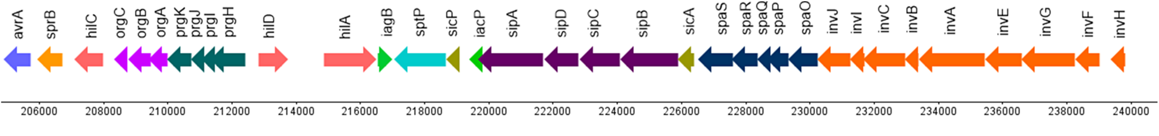
Figure 9:Genetic representation of the Salmonella enterica subsp. enterica serovar Stanley pathogenicity island-1.
The arrows present genes and their orientation, on the x-axis are the genome coordinates.
Credits: CC BY 4.0 modified from Ashari et al. (2019).
Genome assembly strategies
In the early days of DNA sequencing, generating sequencing reads was very costly and slow. Much effort was therefore spent on developing methods requiring the minimum amount of sequence data to assemble a genome. Parts of the genome to be sequenced were cloned into bacterial vectors and amplified that way. These large fragments (much longer than the read length) were then sequenced starting from one end. Next, new sequencing primers were generated from the end of the sequenced part for the next round of sequencing, until the end of the fragment was reached. This rather tedious approach was not feasible for larger genomes. This led to the development of the whole genome shotgun sequencing method, made possible by the growth in compute power for assembly. Here the cloned DNA fragment is sheared into smaller fragments which are sequenced all at once. With the advent of 2nd generation sequencing, this was updated by leaving out the cloning step. 2nd generation sequencing technology (e.g., Illumina) allows for a mixture of fragments to be sequenced at the same time and the volume of sequencing data generated is large. So instead of requiring lab work to select which section to sequence, everything is sequenced at once and the puzzle is solved later computationally.
Whole genome sequencing
Nowadays, the most widely employed genome sequencing approach is whole genome sequencing (WGS, Figure 10). As the term implies the whole genome is sequenced, without discrimination. DNA is extracted from cells and sheared into random fragments. These fragments are then size selected and sequenced using Illumina, PacBio or Oxford Nanopore technology, or a combination. Note that for larger eukaryote genomes WGS generally generates draft genome assemblies; additional steps are required to gain a complete, high-quality reference genome assembly. On the other hand, bacterial assemblies from long reads are usually complete.
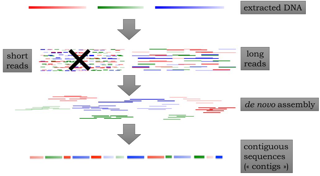
Figure 10:Whole genome sequencing and assembly.
Short reads on the left are generally not used anymore for de novo assembly,
apart from prokaryotes and viruses. Also, many of the available reference genomes
have been generated this way. Contigs refer to the longest stretches of the genome that
can be assembled without ambiguity (see also repeats)
Credits: CC BY-NC 4.0 Ridder et al. (2024)
Assembly challenges
The main challenge of assembly is to reconstruct the original genome sequence from the millions or billions of small reads. Some people have compared this process to putting a stack of newspapers (each newspaper representing one copy of the genome) through a shredder and attempting to reconstruct a single original newspaper from the resulting confetti. Solving this puzzle has driven the development of dedicated assembly algorithms and software. Any computational approach has to overcome the real-world challenges posed by the sequenced data and the characteristics of genomes.
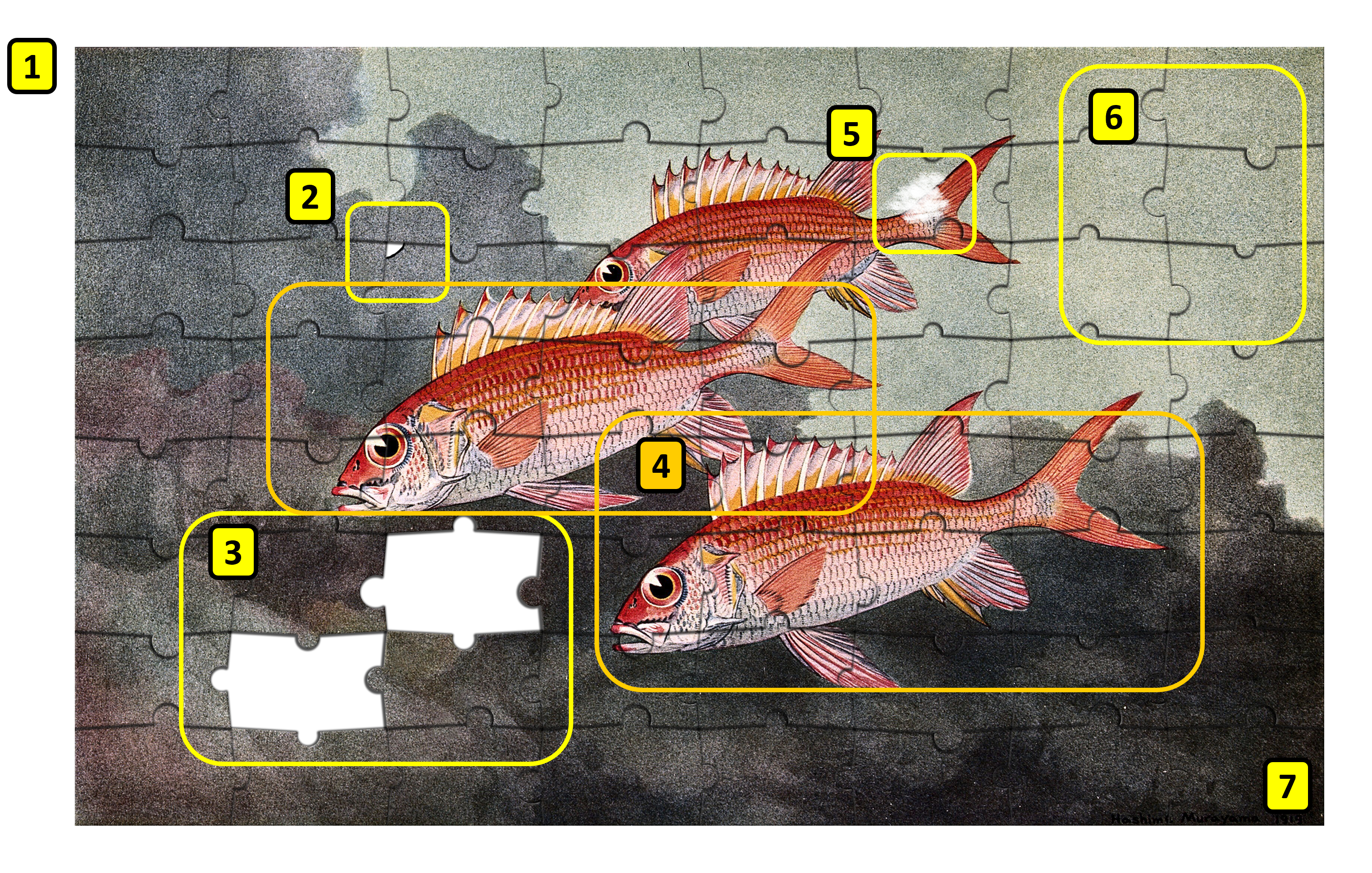
Figure 11:The assembly problem as a jigsaw puzzle. Numbers are referred to in the text below. Credits: Based on Public Domain Mark Murayama (1919), CC BY-NC 4.0 Ridder et al. (2024).
If we look at a genome assembly using the analogy of a jigsaw puzzle (Figure 11), the challenges become obvious:
There is no picture on the puzzle box, i.e., we have no idea what the assembled genome is meant to look like. We can look at related genomes, but this will only give an approximate idea (Number 1 in the image).
There are loads of pieces in the puzzle, billions of them. Every piece represents a small part of the genome that has been sequenced.
Some pieces are frayed or dirty, i.e., reads contain errors, further obfuscating the overall picture (2 and 5).
Some pieces are missing. Some parts of the genome do not break as easily as others, and are not included in the sheared fragments. Others have extreme GC values and do sequence less efficiently. (3)
Some parts of the puzzle contain the same image. In genome terms, these are duplicated regions, where some genes may have more than one copy. For example, the ribosomal RNA cistron (the region which encodes the parts of the ribosome) consists of multiple copies (4).
Some parts of the puzzle look completely identical and are featureless: the repeat regions (6).
In circular genomes, there are no “corners”: we do not know where the genome begins or ends (7).
In addition to the metaphors of the single puzzle, many organisms contain two (i.e., diploid) or more (i.e., polyploid) copies of the same chromosome, with small differences between them. In essence, in this case we try to assemble one puzzle from two (or more) slightly different versions. If these differences grow too big, parts from the two puzzles may be assembled independently without noticing (remember - we have no puzzle box!).
With long high-quality reads this puzzle challenge becomes simpler, as there are fewer pieces in total and fewer featureless parts. Currently, chromosome-level assemblies are routinely generated using PacBio HiFi reads in combination with other technologies.
Repeats
Mainly eukaryote genomes contain sequences that have many, near-identical copies along the genome. These repeat regions (in the puzzle analogy, the background) are the main challenge in genome assembly and most contigs (contiguous sequences, the longest stretches that can be assembled without ambiguity) stop at the edges of repetitive regions. Given the near-identical nature or repeat sequences it is difficult for assembly software to determine which read belongs to which repeat element copy. The evidence used is at the edge of a repetative sequence where it overlaps with non-repetitive sequence. The process is like finding many puzzle pieces containing both bits of fish and background, and trying to figure out which edge belongs to which fish and how much background goes in between. One solution for solving the repeat problem are longer reads (that can bridge the sea between two fishes). To illustrate the scale of the problem that repeats pose in assembly: most mammalian Y-chromosomes have not been assembled for more than 50%, because of the repeat content. Chapter 1 explains how to mask repeats from a genome as a first step prior to genome annotation.
Assembly quality assessment
When assembling a new genome, we have no way of verifying its quality against a known ground truth. We also rarely get a complete genome or chromosome as a single contig as a result. Therefore, other metrics and methods are required to assess the quality of an assembly. We can use the experience gained in other assembly projects to gauge the quality of an assembly; we can compare it to closely related genomes that have already been assembled; and we can compare the assembly with the expectations we have about the genome in terms of overall size, number of chromosomes and genes, given the known biology of the species.
Structural and functional annotation
The next step after genome assembly is annotation. First, during structural annotation we try to identify the location and structure of (protein coding) genes (see chapter 1 - Gene prediction). Next, we attempt to identify the function of the predicted gene during functional annotation (see chapter 1 - Functional annotation).
Insights from complete genomes
The contiguity and completeness of an assembly determines what we can learn from them. In the reference genome quality section, co-segregating alleles and gene order were already mentioned. If a genome is assembled in fewer, larger pieces (i.e., longer contigs), we can also understand more about the long distance regulatory elements that play a role in regulation of gene expression (Figure 12).
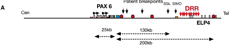
Figure 12:Physical map of the human PAX6 locus showing long distance regulatory elements. The DRR region regulates the expression of PAX6, the red dots show the exact locations of the regulatory elements. The dotted arrows show the distance in kilo bases between those regulatory elements and PAX6. Credits: Kleinjan et al. (2006)
As discussed above, the telomere-to-telomere assembly of the human genome added the 5% hitherto missing genome sequence. While the previous human genome assembly was already considered gold standard and very complete, the number of genes increased with 5%, of which 0.4% were protein coding. This increase in identified genes also allows the study of expression patterns of these genes. An increase in genome coverage can also reveal hidden elements. As an illustration, Figure 13 shows all paralogs of a disease related gene that have finally been resolved. Most of the missing copies were in hard to sequence parts of the genome. Chromosome-level assemblies also allow us to study genome evolution itself, the way chromosomes are rearranged during evolution and speciation.
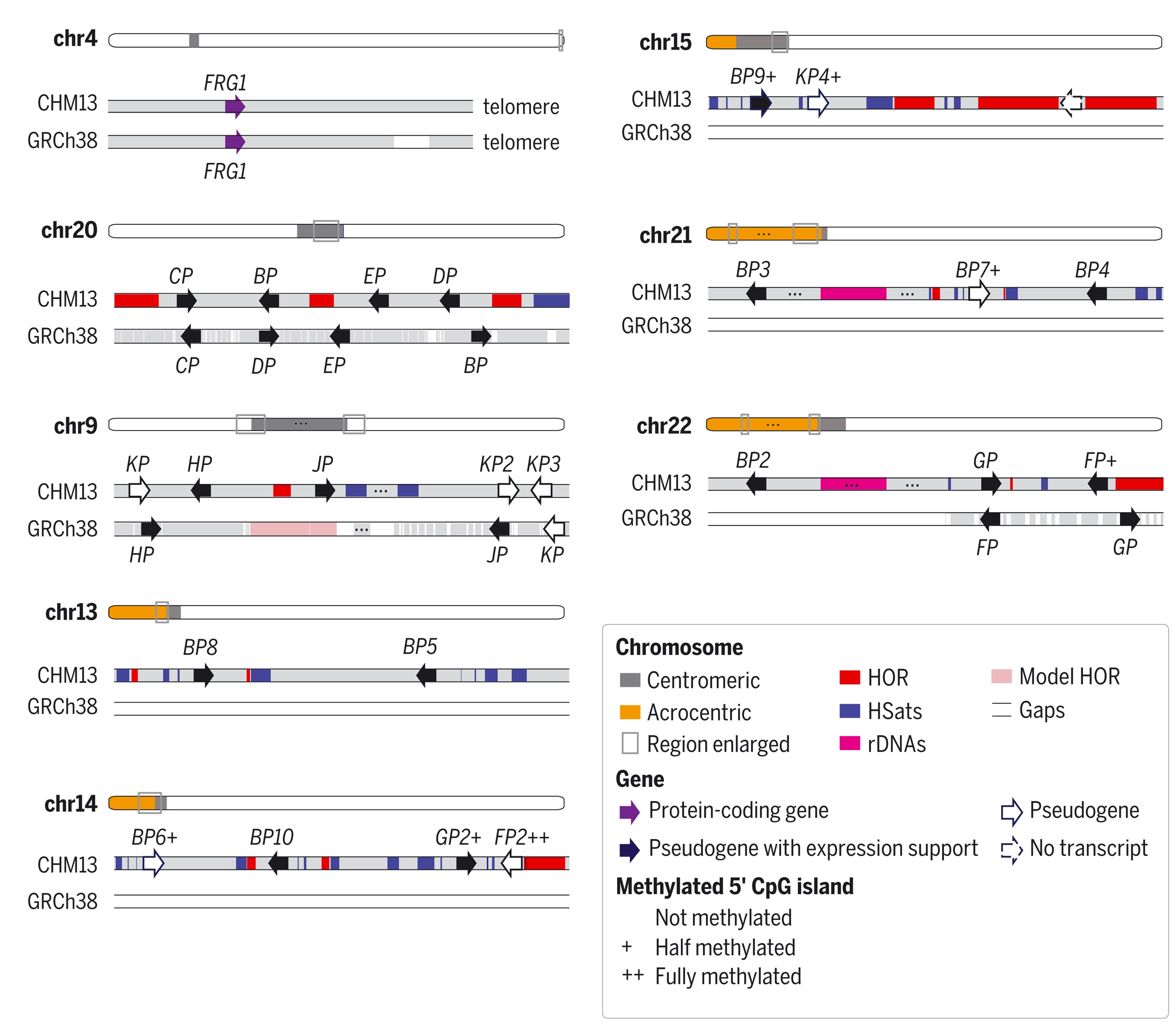
Figure 13:The protein-coding gene FRG1 and its 23 paralogs in CHM13. Only 9 were found in the previous assembly (GRCh38). Genes are drawn larger than their actual size, and the “FRG1” prefix is omitted for brevity. All paralogs are found near satellite arrays. FRG1 is involved in acioscapulohumeral muscular dystrophy (FSHD). Credits: modified from CC BY 4.0 via PMC Nurk et al. (2022).
Variants
When a (closely related) reference genome is already available, reads can be mapped to that genome. Mapping entails finding the location in the genome that matches each read, allowing for some small differences - genomic variation. Such variation can help explain phenotypic variation (see Box 5.3). Genomic variation between samples, individuals, and/or species can also be used to study evolutionary history (see also chapters 2 and 3, on multiple sequence alignments and phylogeny). Variants are divided into two main groups: structural or large-scale variants and small-scale variants. First, we will focus on small-scale variants. Within this group we distinguish single-nucleotide polymorphisms (SNPs), multiple nucleotide polymorphisms (MNPs) and small insertions and deletions (indels):
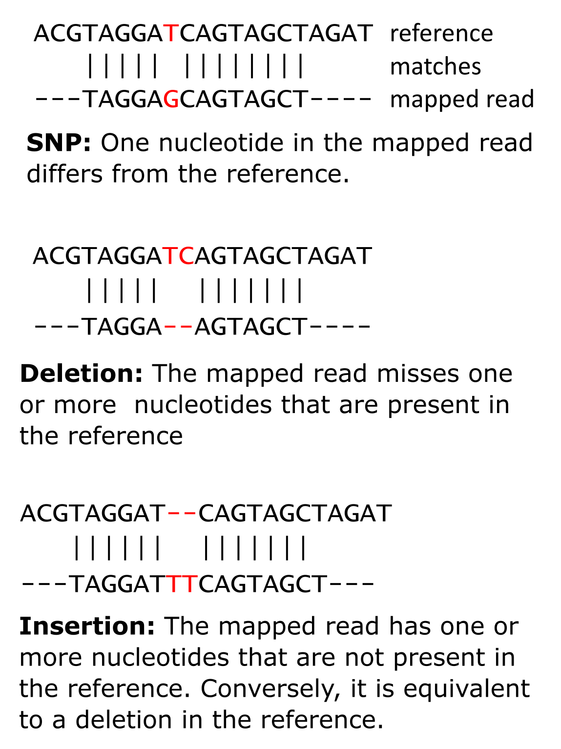
Figure 15:A single-nucleotide polymorphism (top left), an insertion (bottom), and a deletion (top right). Credits: CC BY-NC 4.0 Ridder et al. (2024).
Each variant at a particular position of a reference genome is called an allele. In our example of a SNP above (Figure 15), we have a reference allele T and an alternate allele G. With regards to SNPs, when a sample originates from a single individual, the theoretical number of alleles at any position of the reference cannot exceed the ploidy of that individual: a diploid organism can at most have two different alleles (as in our example), a tetraploid can at most have four, etc. Given that we only have four different nucleotides, the maximum number of possible alleles for a single position is four, for higher ploidy alleles get complicated. But if we find more than two alleles in a diploid organism it must be the result of an error, either in the read or in the reference. In rare cases it can be the consequence of heterogeneity between cells, e.g. in cancer.
Variant calling
As we have already seen, variants can be real, they can be the result of sequencing errors, or represent errors in the reference sequence. The process of detecting variants (SNPs and indels) and determining which are real or most likely errors is called variant calling. To indicate the probability that a variant is real, a quality score is assigned to each variant. This considers the coverage and the mapping quality (i.e. how well the read matches the reference) at the position of a putative variant. Variant calling software will also report, among a whole range of statistics, the so-called allele frequency (AF), determined by the proportion of reads representing each allele from all reads that map . In a diploid organism with one reference allele and one alternate allele we expect both, on average, to have a frequency of 0.5. When the frequency of one allele is close to 0, it is an indication that this variant is most likely due to an error.
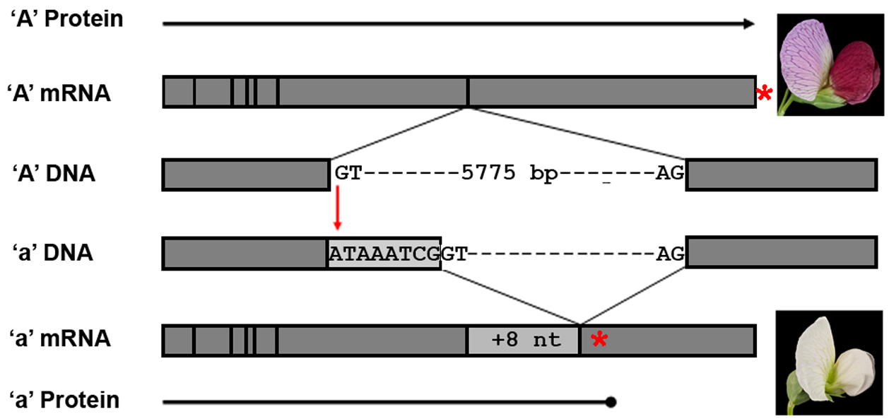
Figure 16:The main features of the bHLH gene and its expression products (not to scale). In Caméor, a white flowered pea cultivar of genotype a, there is a single G to A mutation in the intron 6 splice donor site that disrupts the GT sequence required for normal intron processing. In the DNA, exons 6 and 7 are shown as grey boxes that flank the intron 6 splice donor and acceptor sequences. In the RNA, the vertical lines represent exon junctions, and the light grey box represents the 8 nucleotide (nt) insertion in the a mRNA that results from mis-splicing of intron 6. The red stars show the position of the stop codon in the predicted protein, highlighting the premature termination in the white flowered cultivar. Credits: CC0 1.0 Hellens et al. (2010).
Variants and their effects
SNPs between individuals underly most phenotypic variation. Sometimes a single variant causes a different phenotype, like the classical mendelian trait of flower color (Figure 16). More often phenotypic traits are the result of multiple variants, one example is height (in humans, height is determined by >12000 SNPs Yengo et al. (2022)). Some variants can cause hereditary defects or increase the risk of certain diseases. Well-studied examples are mutations in the BRCA1 and BRCA2 genes (Figure 17). A specific mutation in the BRCA1 gene increases the chance for that person to develop breast cancer during their lifetime to 80%.
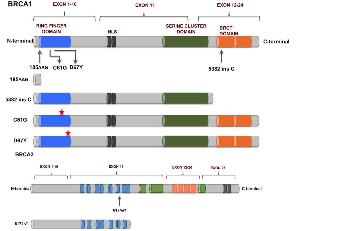
Figure 17:Mutations in BRCA1 and BRCA2 found in breast and ovarian cancers. Credits: CC BY 4.0 Mylavarapu et al. (2018).
Large-scale genome variation
Above, we discussed small scale variants such as SNPs and indels. In contrast, large-scale variants are structural variants where parts of genomes have been rearranged, duplicated or deleted (Figure 18). A special case is copy number variation, where genes (or exons) have been duplicated.
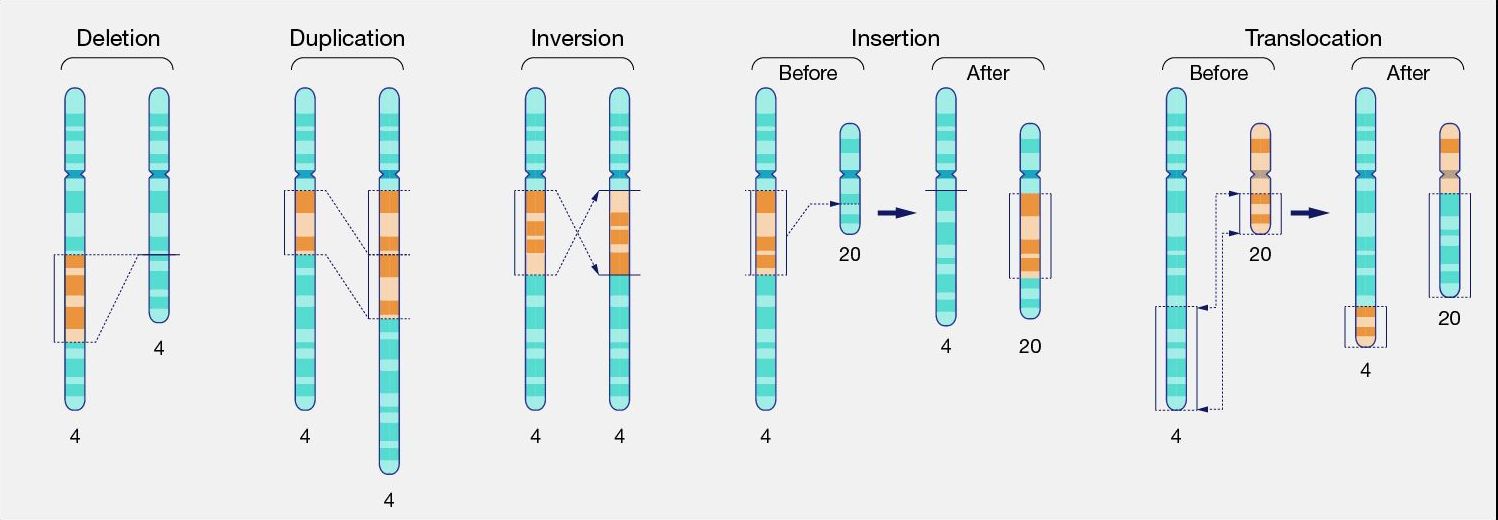
Figure 18:Different types of structural variants on chromosome level. Credits: CC0 1.0 National Human Genome Research Institute (2024).
Structural variation
Structural variants are variations that are larger than approximately 1kb in size, which can occur within and between chromosomes. Structural variants have the potential to have major influence on phenotypes, such as disease, but that is not necessarily the case. Structural variants do appear to play a large role in the development of cancerous cells.
Copy number variation
Copy number variants (CNVs) are a special case of structural variants where the number of times a gene occurs on the genome changes. In a diploid organism, a deletion will leave only one copy, whereas a duplication can result in three or more copies of the gene in an individual. Changing the copy number can be part of normal variation in a population, e.g., genes involved in immune response vary in copy number; but, more often than not, copy number variation leads to severe phenotype changes, such as diseases in humans.
Detection of structural variants
Accurately detecting structural variation in a genome is not easy. The challenge lies in detecting the edges of the variants (the so-called breakpoints) and, in case of duplications/insertions/deletions, the resulting copy number. When a mapping-based approach is used (possible if the reference genome is known) we can use read depth and paired end reads to detect variants. More copies of the gene in the sample will result in more reads from that gene (Figure 20) than expected for a single copy. Conversely, coverage is expected to drop when one copy of a gene is lost.
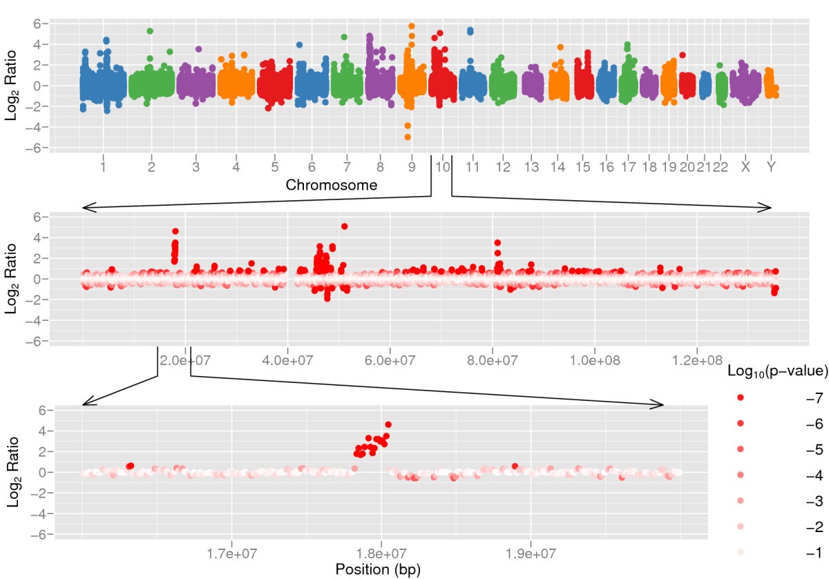
Figure 20:Gene duplication results in higher coverage than expected in the duplicated regions. Credits: CC BY 2.0 Xie & Tammi (2009).
Orientations of paired end reads as well as split reads (reads where on part maps to the inversion and the other part to surrounding sequence, similar to Figure 28) are good indicators to detect the boundaries of inversions, but also substitutions and translocations. The rearrangements will result in one read from a pair mapping to one genomic location and the other read to another location. Reads overlapping the breakpoint will be split in the alignment.
Examples of structural variants and CNVs
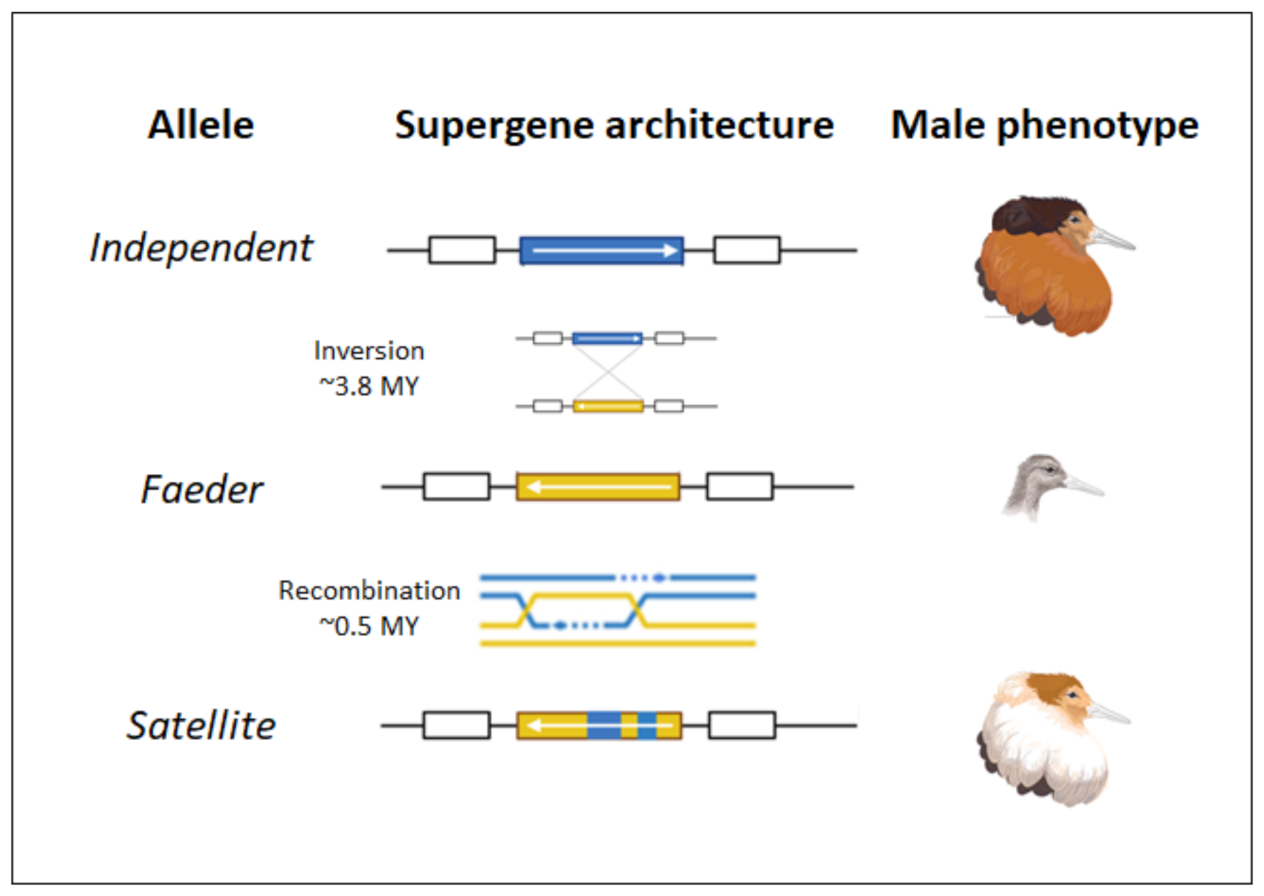
Figure 21:Orientation of the inversion in the three male morphs. Credits: CC BY 4.0 Baguette et al. (2022).
Large chromosomal inversions play a role in within-species phenotypic variation and have also been found as the result of introgression after hybridisation of two different species. One example of a within-species inversion yielding large phenotypic differences are the three male morphs in the ruff (Calidris pugnax, Figure 21).
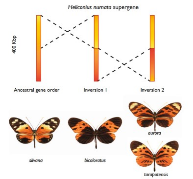
Figure 22:At least two genetic inversions are associated with the Heliconius numata supergene. The ancestral gene order, which matches that in H. melpomene and H. erato, is shown on the left and is associated with ancestral phenotypes such as those found in H. n. silvana. Two sequentially derived inversions are associated with dominant alleles and are shown in the middle and right. Credits: CC BY 4.0 Jiggins (2017).
Another example is the acquisition of an inversion containing genes for wing color patterns in different species of Heliconius butterflies (Figure 22). Copy number variation can also affect phenotypic traits with an example being flowering time, photoperiod sensitivity, and height of wheat plants (Figure 23).
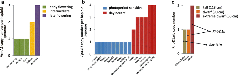
Figure 23:Gene CNV contributes to wheat phenotypic diversity. a) CNV of Vrn-A1 gene controls flowering time by affecting vernalization requirement; b) CNV of Ppd-B1 controls flowering time by affecting photoperiod sensitivity; c) CNV of Rht-D1b gene (a truncated version of Rht-D1a) determines severity of plant dwarfism phenotype. In all three cases, the impact of gene copy number on observed phenotype has been verified experimentally. Source data: a, b, Díaz et al. (2012); c, Li et al. (2012). Credits: CC BY 4.0 Żmieńko et al. (2013).
Functional genomics and systems biology
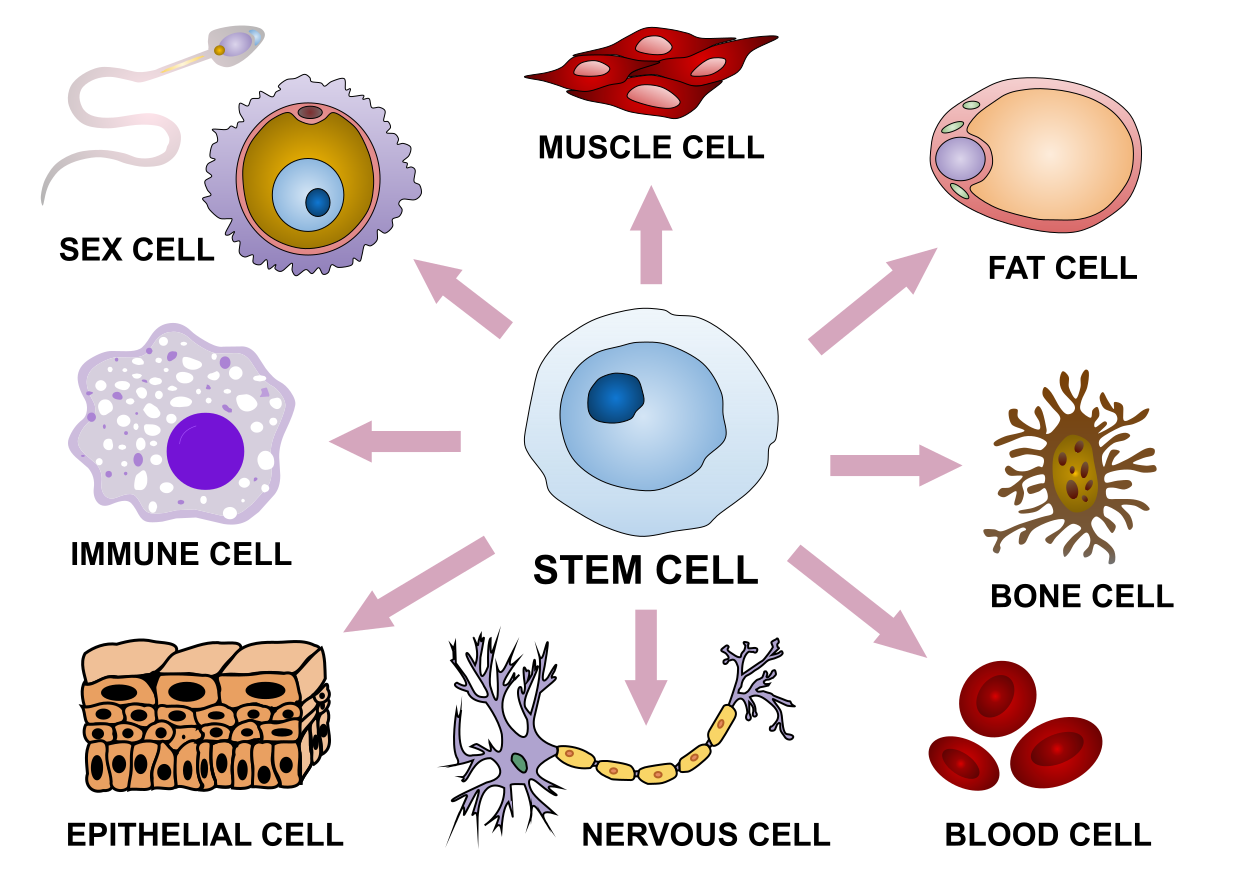
Figure 24:With the same genome, human stem cells differentiate into a wide range of shapes. Credits: CC BY-SA 4.0 Fournier (2019).
The need for functional genomics
While genomics provides us with an enormous amount of data on genomes and genes, it is clear that these are only part of the story. Cells are not static objects: they display different behaviour during their lifetime, and react to changes in the environment and to signals from other cells. In most multicellular organisms, cells in different organs develop in very different ways, leading to different cell shapes, tissue organization and behaviour (Figure 24). Still, each cell contains the same genome, so there must be differences in the way which that genome is used. In other words, if the genome is the book of life, it must also contain the information on how to read it.
A part of the explanation lies in what is called epigenetics, modifications of the genome that do not change the DNA sequence but do influence gene expression (Box 5.5). There are other mechanisms besides epigenetics that control how genes are expressed, and how the resulting proteins eventually fulfil their function in the cell. The most well-known ones are interactions between proteins and DNA (transcription factors and enhancers, influencing expression); interactions between proteins, to form complexes or to pass signals; and catalysis of metabolic reactions by enzymes.
The field of research that studies how genes are used is called functional genomics. The most prominent functional genomics project started immediately following the completion of the human genome: the ENCODE (“Encyclopedia of DNA elements”) project (2005-2015), aiming to identify all functional parts of the genome.
The role of omics data
Functional genomics research mostly measures cellular activities in terms of the abundance of genes, proteins and metabolites, and the interaction between these molecules. When performed at a cell-wide level, i.e., attempting to measure all molecules of a certain type at once, these are called omics measurements. The technology to measure such omics data is usually high-throughput, which means that little manual work or repetition of experiments are needed. We generally distinguish five main levels of omics measurements as illustrated in Figure 1, although many new omics terms are still being introduced. Next to genomics, the following omics measure:
- Epigenomics: all epigenetic modifications of the genome.
- Transcriptomics: the expression levels of all genes.
- Proteomics: the presence/quantity of all proteins.
- Metabolomics: the presence/quantity of all metabolites.
- Phenomics: the eventual phenotype(s), i.e., form or behaviour, of a cell or organism.
Such measurements are increasingly also applied on mixed samples, mostly bacterial/fungal/viral communities such as found in the human gut and in the soil. As a kind of ‘meta’ analysis, this has been labelled metagenomics, metatranscriptomics, etc.
The introduction of omics technologies over the last 25 years has broadened the field of bioinformatics and made it increasingly relevant to all areas of biology. Very large measurement datasets are now routinely produced and should be cleaned, checked for quality and processed. Moreover, the data should be stored in databases to make it accessible and re-usable for further research. Finally, careful analysis, interpretation and visualization of the data is essential to allow biologists to infer biological functions. Bioinformatics delivers the tools and databases to support all these steps.
Even though omics measurements provide highly detailed overviews of cellular states and reactions to perturbations, there are a number of important limitations:
- Experimental cost: omics devices are often expensive to acquire, and each experiment requires labour and consumables
- Technical noise: all measurement technologies come with inherent variation and experiment requires labour and consumables
- Biological variation: different cells, organs or individuals will differ in their biological state and make-up
- Bias and coverage: most omics technologies are most efficient (or even only work) for measuring specific types of molecules or interactions
Typically, functional genomics experiments involve studying the effect of genetic variation on certain omics levels. Such variation can be natural, for example comparing omics data measured on two organisms with known (limited) genetic differences due to evolution. It can also be experimentally introduced, for example by introducing small mutations in the DNA sequence, knocking out genes, introducing new genes etc. Variation can also be introduced in the environment, e.g. by changing the temperature, adding or removing nutrients, introducing drugs etc. The effects of such interventions at a specific omics level then provide information on the function of the manipulated gene(s) or the effect of the environment.
From functional genomics to systems biology
Where functional genomics uses omics measurements to learn about the role of genes and proteins in the cell, individual experiments and measurements generally only provide individual pieces of the puzzle, which often do not make much sense without understanding other cellular processes. Recognizing the need for a more holistic approach, systems biology was proposed as a scientific approach in which the main goal is to construct models of living systems, that are increasingly refined by hypothesis formation, experimentation, and model extension or modification.
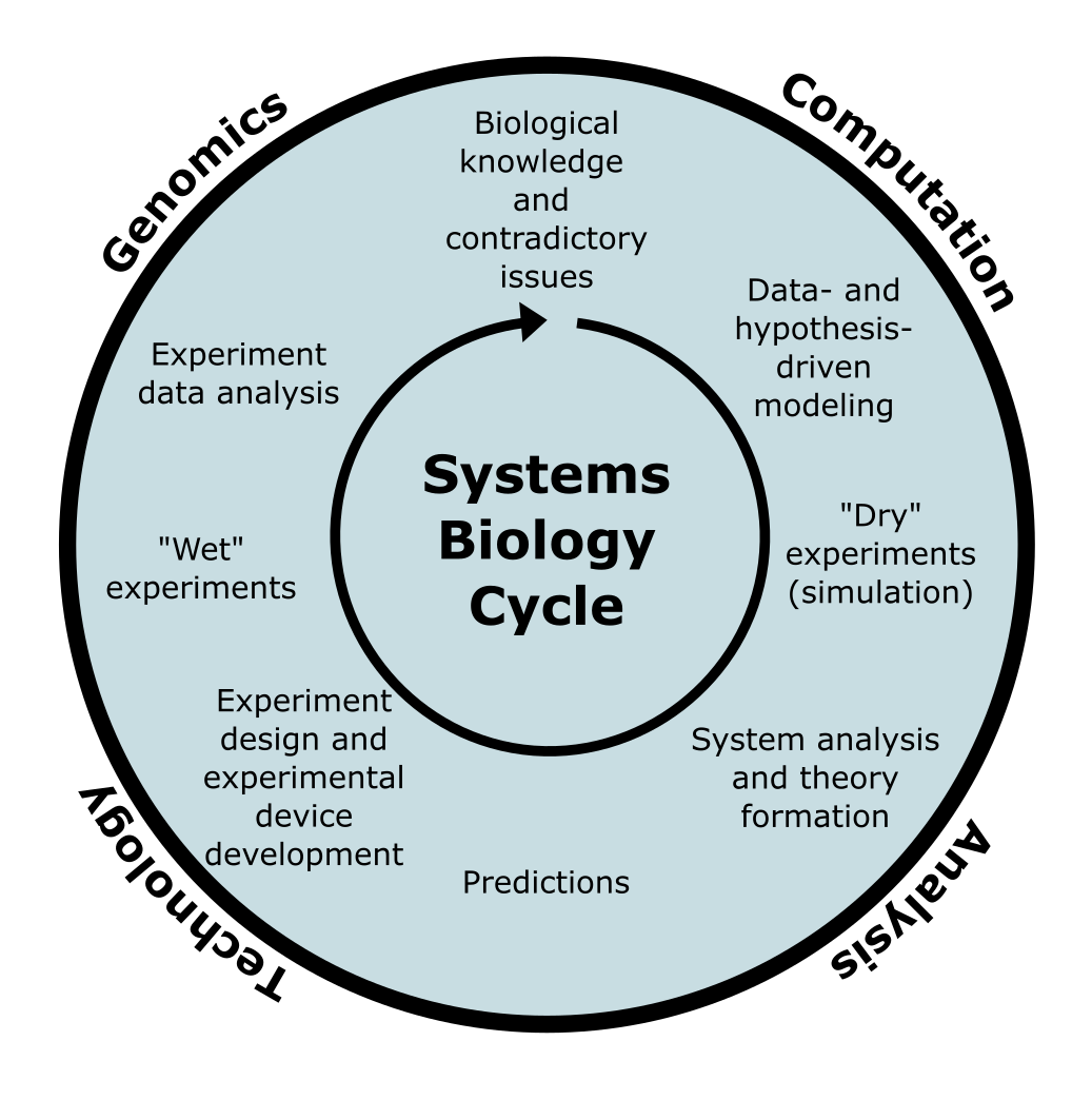
Figure 26:The systems biology cycle, aiming to iteratively improve models of living systems (based on Kitano (2002)). Credits: CC BY-NC 4.0 Ridder et al. (2024).
Eventually, the hope of systems biology is to arrive at systems-level understanding of life that will allow us to simulate the effects of interventions (mutations, drug treatments, etc.) or even (re)design genes and proteins to improve certain behaviour, such as production levels of desired compounds in biotechnology. While we still have a long way to go, omics data analysis is an essential element in systems biology.
Transcriptomics
Transcriptomics is concerned with measuring transcript levels (i.e., the levels of transcription of the genome to RNA). RNA and its role in the cell has already been discussed in chapter 1. Here, we focus on measuring and counting the expression of genes (i.e. mRNA). For the understanding of transcriptome analysis it is important to remember that in eukaryotes most genes contain introns and that one gene can have many alternative transcripts.
In transcriptomics, the aim is to measure presence and abundance of transcripts. Such measurements are based on a large number of cells, but more recently the transcriptome of individual cells can also be studied. So what do transcripts and their abundance tell us about a studied subject? In any experiment we often want to know what happens to a cell/tissue/organism under certain circumstances. Most informative for this are protein levels and even more specifically protein activity, as these directly influence what happens. As will be discussed below, detecting and measuring proteins is complex. Measuring mRNA levels is far easier, but it is important to realise that they only provide a proxy to what happens in a cell. mRNA levels do not always correlate with protein levels as transcripts can be regulated or inhibited, affecting translation. Protein levels can be equally affected by regulation and abundance does not always correlate with activity.
Despite its limitations, we can address a number of very relevant questions based on transcriptomics measurements. Three general analyses will be discussed below, but note that to detect relationships between experimental conditions and mRNA expression patterns, it is important to be aware what can cause variation in mRNA levels. Some of these causes may be intended variation, some will cause noise.
mRNA levels:
- are the result of mRNA synthesis and mRNA decay
- differ between genes, isoforms, cells, cell types and tissues, and developmental stages
- vary with cell cycle, during the day (circadian rhythm) and/or season
- depend on the environment
How to measure mRNAs?
Just like the study of genomes, transcriptomics has greatly benefitted from technological developments that allowed an increase in throughput and sensitivity of measurements. If you are interested, Box 5.12 and Box 5.13 provide an overview of technologies that were important for the development of the field (such as microarrays), but are not widely used anymore; at this time, RNAseq is almost exclusively used to measure mRNA levels.
Note that microarrays haves now been mostly superseded by RNAseq as a cheaper and better quality alternative (see below). However, there are many microarray samples still available for re-use in databases, as submission of measurement data to such databases is compulsory upon publication of a scientific paper. The most well-known repositories are the NCBI Gene Expression Omnibus (GEO), with as of March 2024 ~7.1 million samples, and EBI ArrayExpress. If you are interested in a certain question that may be answered using transcriptomics, it makes sense to look here first to see what experimental data is already available. Note that the technology used determines how the expression level should be interpreted (see box below).
RNAseq
RNAseq makes use of affordable and reliable sequencing methods. Important for the development of RNAseq was the reliable quantitative nature of NGS protocols and sequencers. RNAseq is untargeted: all RNA in a sample can in principle be sequenced and it is not necessary to have prior knowledge of transcript sequences. While RNAseq is mainly used to study transcript abundance, it can also be used to detect transcript isoforms (and their abundance), as well as variants (see Variants above).
Protocol
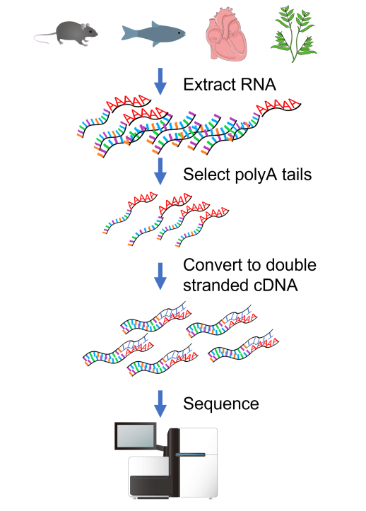
Figure 27:Standard RNAseq protocol. Credits: CC BY 4.0 Ridder et al. (2024) modified/created from CC BY 4.0 DataBase Center for Life Science (DBCLS) (2011), Spedona (2023), Christinelmiller (2020), CC BY 3.0 Life Science (DBCLS) (2013), Servier (2016), CC0 1.0 Ingo (2014).
The standard protocol of an RNAseq experiment is shown in Figure 27. First, all RNA (total RNA) is extracted from a biological sample. Next, mRNA is selected using a polyT oligo to select RNA with a polyA tail. The RNA is then converted to stable double stranded cDNA. The resulting cDNA library is then sequenced, usually as paired end reads of 100-150bp. A standard sequencing run results in 30 million or more reads per sample.
The read lengths currently used are relatively short and complicated methods are required to assign reads to exons and isoforms. New developments in this field are long cDNA conversions that allow sequencing of full-length transcripts on PacBio and direct sequencing of RNA on Oxford Nanopore. This allows the detection of the actual isoforms present in samples.
Next, the reads need to be assigned to their corresponding transcripts. For this there are two options: mapping of the reads to an existing reference, which can be either a genome or a transcriptome; or a de novo assembly of the transcripts (similar to assembly of genomes). Once reads have been assigned to their corresponding transcript or gene, expression is quantified by counting the number of reads per feature.
The advantage of not using probes (compared to qPCR and microarrays) is that RNAseq works for species without a reference genome, can identify alternatively spliced transcripts, SNPs in transcripts, etc. A challenge is that usually large datasets are generated, which require dedicated analysis workflows.
Mapping
In principle, sequenced reads from an RNAseq experiment do not differ from reads sequenced from genomic DNA in that they can be mapped to a reference sequence. The same algorithms apply when mapping RNAseq reads to an assembled transcriptome (a reference sequence that only contains RNA sequences) or to prokaryotic genomes.
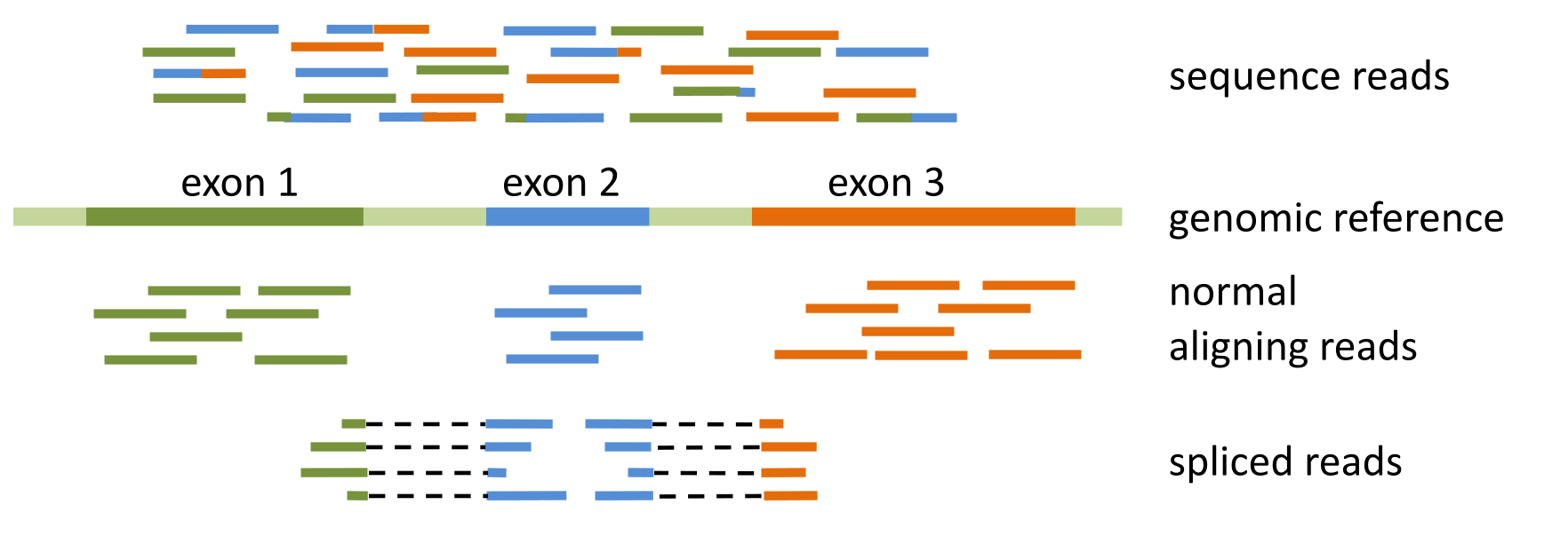
Figure 28:Spliced mapping of mRNA reads to genomic reference with splice-aware aligner. Credits: CC BY-NC 4.0 Ridder et al. (2024).
Mapping eukaryotic mRNA sequences to a genomic reference is more cumbersome, as most genes have introns, which are no longer present in the mature mRNA (Figure 28). This means that reads might contain an exon-exon junction and should be split along the reference, so-called spliced mapping. Most aligners will not consider this a valid option. Special splice-aware aligners have been developed for this reason, that are able to map normal reads that map contiguously to the reference sequence as well as reads that are split across splice sites (Figure 28). They also take into account known intron-exon boundaries to determine the point within a read where it has to be split and whether the split alignment is correct.
Transcript quantification
After sequencing and mapping, the next step is to quantify the abundance of transcripts, i.e., the expression levels. Reads assigned to each feature (exon or gene) are counted, with the underlying assumption that the number of reads mapping to a feature is strongly correlated with the abundance of that feature in the experiment. Comparing abundance of transcripts between samples, conditions and experiments is not as straightforward as it seems. Apart from the bullet points above that influence mRNA abundance, there is variation in each sequencing experiment. The main variation affecting comparability of read counts between samples is the total number of reads sequenced in each sample. Also, not all transcripts are the same length, affecting the number of reads detected per transcript. So, some normalisation is required to take into account these differences and make data comparable. The main methods are:
Simple counting: this is the starting point of every analysis. We count the number of reads that map to each exon or gene.
CPM: counts per million (reads), a relative measure for the read counts corrected for the total number of reads of a sample. It assigns each read a value that corresponds to the proportion of the total number of reads that single read represents. This tiny fraction is then multiplied by a million to make it more readable.
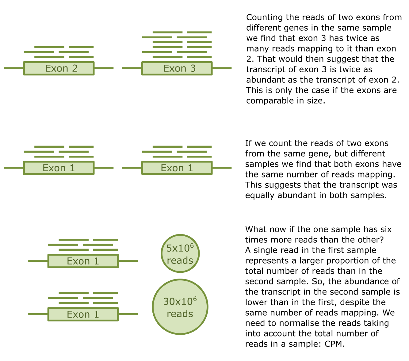
Figure 29:Credits: CC BY-NC 4.0 Ridder et al. (2024).
- RPKM, FPKM and TPM: when comparing expression of two different transcripts, we also have to take into account the characteristics of the transcripts we are comparing and normalise accordingly. RPKM and FPKM (Reads/Fragments per kilobase transcript per million) normalise the counts per feature length and the total number of reads. TPM (transcripts per million transcripts) normalises per transcript. TPM uses a calculation to give a measurement of which proportion of the total number of transcripts in the original sample is represented by each transcript.
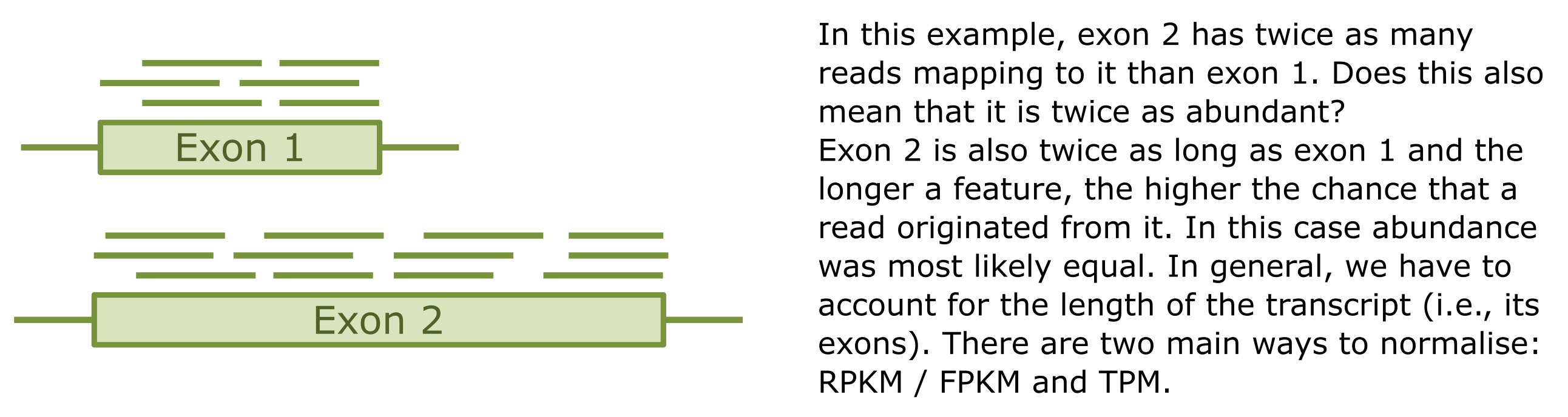
Figure 30:Credits: CC BY-NC 4.0 Ridder et al. (2024).
There is no clear optimal method, and there is a large debate whether RPKM/FPKM or TPM are preferred. CPM can clearly only be used when there is no difference in transcript length, e.g., when comparing one transcript between two samples.
Proteomics
As mentioned earlier, transcriptomics is widely applied but does not reflect the overall cellular state accurately. The resulting proteins are the workhorses of the cell, and knowing their concentrations, modifications and interactions provides more insight than gene expression can provide. Unfortunately, while major advances have been made in proteomics technologies, accurate measurement of proteins is still complex and costly, for a number of reasons:
- Obviously, the problem of identifying molecules with 20 building blocks (amino acids) is harder than that of identifying molecules with 4 building blocks (nucleotides).
- Moreover, given alternative splicing, the number of proteins that needs to be distinguished is higher than the number of genes.
- Proteins can be modified in a myriad of ways after translation, structurally, as well as biochemically, by the addition of many different groups on individual amino acids. For some proteins, it is estimated that many thousands of different variants can be found in a cell.
- Most proteins are structured, some form complexes or insert into the membrane; such structures often have to be removed to allow accurate measurements.
- Proteins lack properties that make DNA and RNA easy to multiply (PCR) and measure: replication and binding to complementary strands.
- The dynamic range of protein abundances is enormous: some protein concentrations are a million-fold higher than that of others. This would not be a problem if we had a protocol to make copies of low-abundant proteins (like PCR for DNA), but such a protocol is not available.
Still, a number of methods to measure proteins and their interactions are in use. We distinguish between quantitative proteomics (measuring presence/absence and levels of proteins) and functional proteomics (measuring protein interactions with other molecules).
Quantitative proteomics
While a number of older, gel-based techniques have been used to measure protein absence/presence and even levels, these have been superseded by mass spectrometry (MS) devices. These have been in constant development and improvement since their inception in the late 19th century, and have now reached accuracy levels that allow to study molecules of a wide range of sizes, also including metabolomics. They differ in specific setup, but all follow three basic steps:
- Ionize a molecule.
- Separate or select molecules based on their mass.
- Detect time and/or location of arrival at a detector to infer the mass of each molecule.
To be fully correct, MS measures the mass-over-charge ratio (m/z) rather than the actual mass, i.e., the mass in relation to the charge number of the ion.
For each step, different technologies are available which are best suited to detection of specific mixtures, compounds of interest (proteins, metabolites), and compound size ranges. Figure 31 illustrates a number of widely used separation steps, i.e., by measuring time-of-flight or susceptibility to deflection by magnetic fields or by tuning an oscillating electrical field to allow only specific masses to pass through.
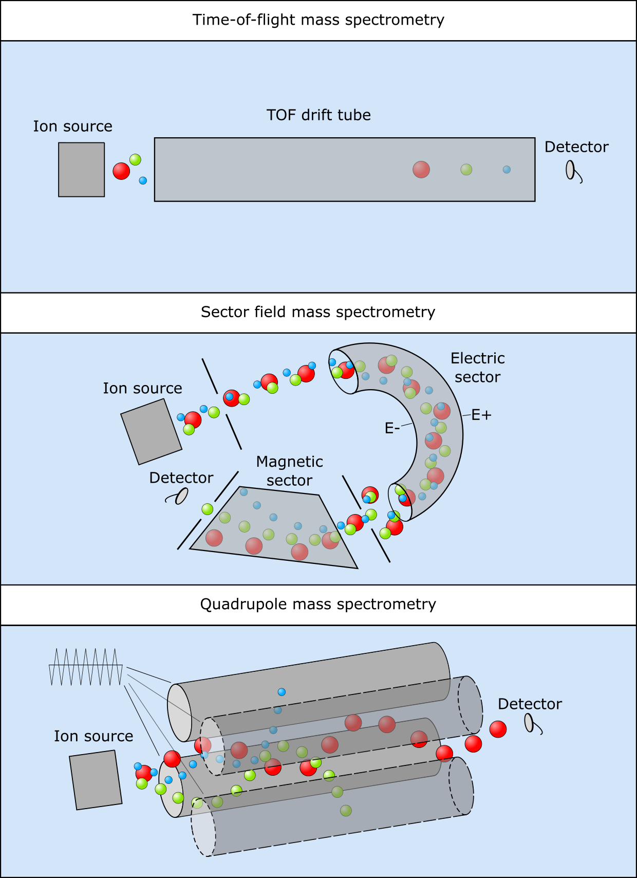
Figure 31:Three mass spectrometry setups, (top) time-of-flight, (middle) sector field and (bottom) quadrupole. Credits: CC BY-NC 4.0 Ridder et al. (2024).
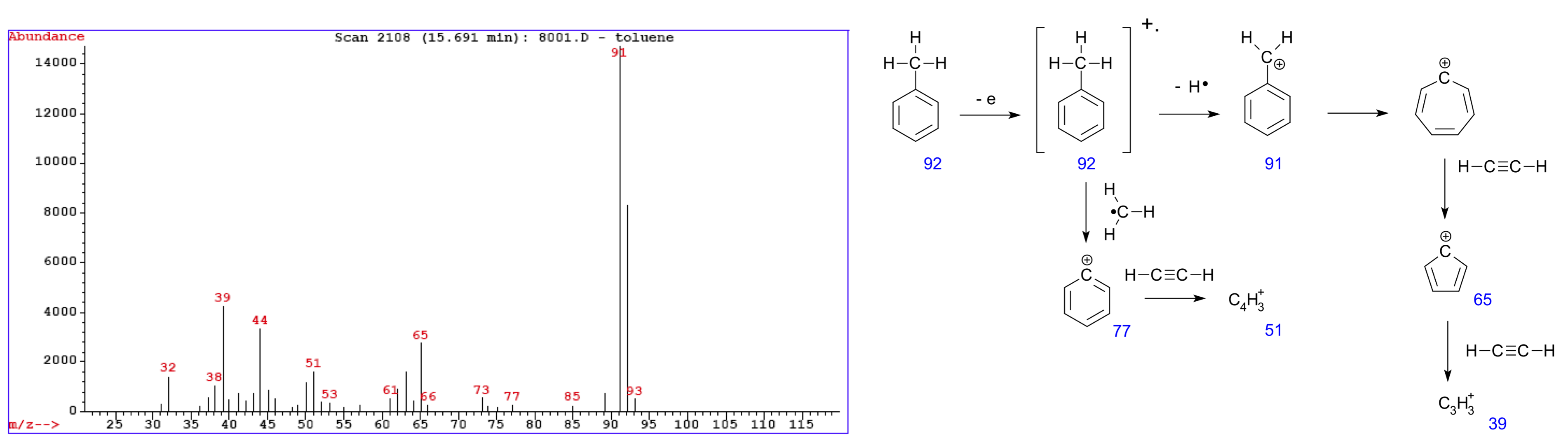
Figure 32:An example mass spectrum measured on toluene (left). The various peaks correspond to fragments of the original molecule (right). Credits: modified from (left) CC BY-SA 3.0 Paginazero (2005), (right) CC BY-SA 3.0 V8rik (2008).
The output of any MS experiment is a mass spectogram, with m/z ratios on the x-axis and peaks indicating how many molecules of a certain mass have been detected (Figure 32).
In theory, if a database of known molecule formulas (e.g., proteins or peptides) and their calculated masses would be available, one could look up each mass and identify the corresponding molecule. A major challenge in interpreting such a spectrum is the limited resolution of MS devices, which means that a certain peak can still be caused by many different types of molecules. Some smaller molecules of interest may even have identical masses (e.g., isoforms) and so cannot be distinguished, which is particularly hard in complex mixtures. A number of extensions try to solve this problem; these are explained in more detail in Box 5.14.
Of particular interest in bioinformatics is shotgun proteomics, essentially similar to shotgun genomics. Specifically for proteins, this is a protocol in which an enzyme is first used to cut the protein at specific places (for example, trypsin cleaves the protein into peptides at arginines and lysines) (Figure 33). The peptide masses are then measured and compared to the mass spectra of predicted peptides resulting from a database of known proteins, to identify the protein likely being measured. This approach can also be used to measure posttranslation modifications, as they lead to small (known) shifts in the measured spectra for the modified peptides.
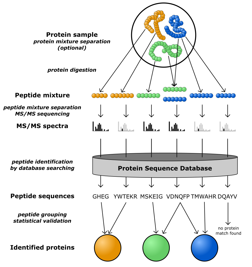
Figure 33:A schematic overview of shotgun proteomics. Credits: CC BY-NC 4.0 Ridder et al. (2024).
Functional proteomics
Next to protein levels, we are also interested in what proteins do in the cell: their functions and interactions. Many protocols and analyses have been developed for this, with most focusing on protein-protein, protein-DNA and protein-metabolite (enzymatic) interactions. Box 5.15 lists some methods to measure such interactions. Note that while many of these experiments are cumbersome, they are essential to advance functional genomics - (bioinformatics) predictions critically depend on high-quality data and cannot replace experimental validation.
Like transcriptomics data, “interactomics” measurements are stored in databases, such as IntAct, and can be used to obtain insights into cell-wide protein interaction networks (Figure 34). Groups of highly connected proteins, i.e., with many interactions, can indicate e.g. protein complexes or signalling pathways within or between cells; protein-DNA relations can be used to identify gene expression regulation programmes.
Note that the methods mentioned measure physical interactions between proteins, as opposed to functional interactions. Such interactions occur when two proteins have similar functions - even though they may never actually physically interact, for example when they are two alternative transcription factors for the same gene. Such functional interactions can be measured to some extent, but are mostly predicted by bioinformatics tools that combine various pieces of evidence: literature, sequence similarity, gene co-expression, etc. STRING and GeneMania are the most well-known examples.
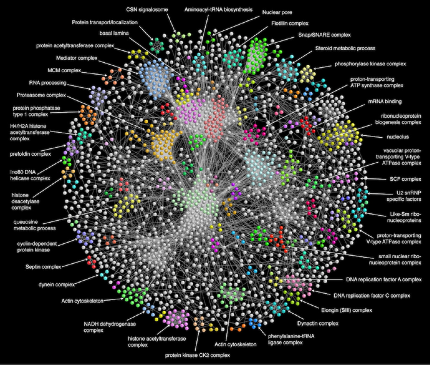
Figure 34:A protein interaction network (4,927 proteins, 209,912 interactions found by tandem affinity purification) for Drosophila melanogaster, with clusters corresponding to protein complexes indicated in color. Credits: modified from Guruharsha et al. (2011) under Elsevier user license.
Metabolomics
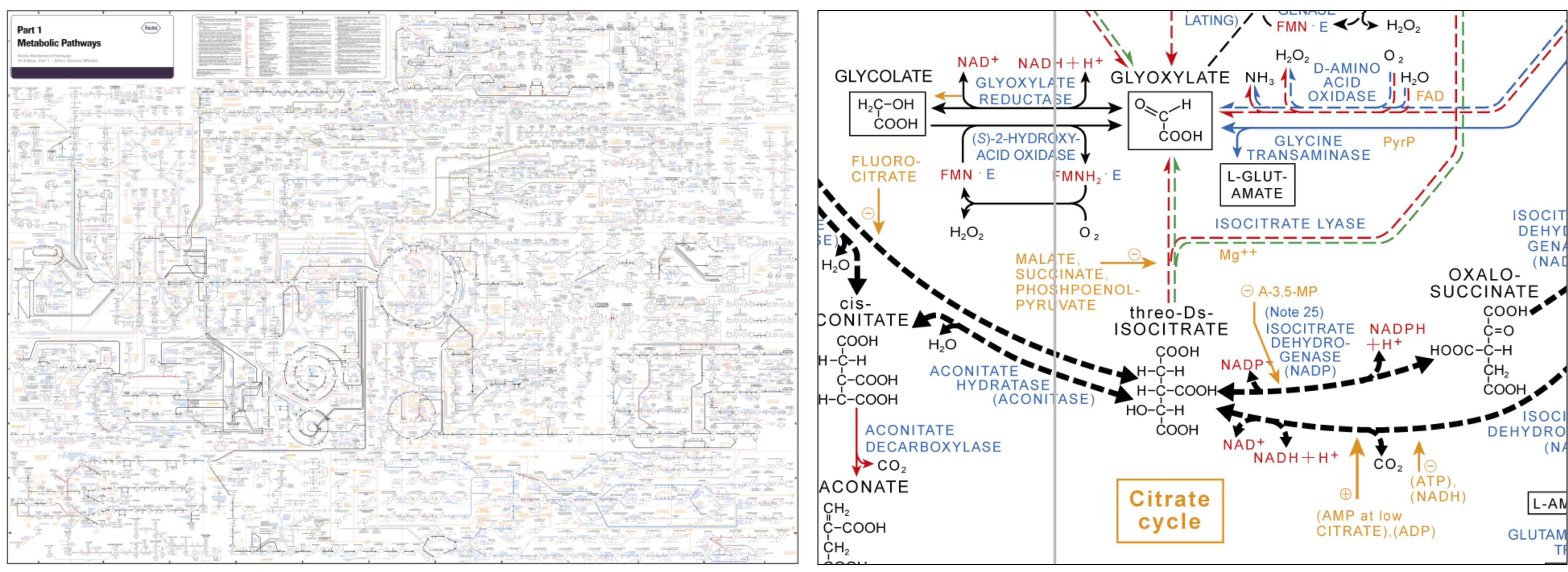
Figure 35:The Roche biochemical pathway chart: global overview of metabolic processes (left) and a close-up of part of the citrate cycle (right). Credits: Roche (2016).
Many cells produce a wide range of metabolites - small molecules or compounds that are part of metabolism. Many of these so-called primary metabolites, serve as building blocks for essential molecules, such as DNA or proteins, and provide energy for reactions. Other metabolites, specialized metabolites, function in many organisms for communication, regulation (hormones), defense (antibiotics), and symbiosis. Some metabolites also regulate relevant phenotypes. As such, solving the structures of all molecules circulating in cells and measuring the concentrations of metabolites as so-called “end points” of cellular organization seems highly relevant in studying growth and development of organisms and communities. Metabolomics is also important in medicine and pharmacology, in food safety and in uncovering the production repertoire of microbes in industrial biotechnology.
For measuring metabolites, mostly the MS technologies described above are employed, in particular GC-MS and LC-MS (see Box 5.14). As the range of metabolite sizes and characteristics is large and many metabolites are still unknown, identifying them from mass spectra is still very challenging. An advantage is that known metabolic reactions, collected in metabolic networks (Figure 35), can support systems biology approaches, specifically in microbes.
Phenomics
The final outcome of cellular regulation is the phenotype, i.e., the set of observable characteristics or behaviours of a cell or organism at macro-scale. These phenotypes often depend in complex ways on levels and interactions of a (large) number of molecules in the cell. Uncovering the genotype-phenotype relation, i.e., what variation at the genomic level underlies (disrupted) phenotypes, is one of the most important goals in many scientific areas, including medicine.
The set of potential phenotypes for different organisms is enormous, and there is no standardized approach to phenomics as there is for the other omics levels. Exceptions include structured databases of human diseases such as MalaCards, and of genetic disorders such as OMIM. Similar approaches are starting to find their way into other areas of biology (ecology, plant development and breeding, and animal behaviour), with (standardized) repositories for image, video, and tracking data. Reliable, high-throughput phenomics data will prove indispensable to make sense of the genetic variation we find.
-Omics data analysis
Transcriptomics, proteomics and metabolomics (can) all provide quantitative measurements on molecule levels present. The resulting data can be analysed in various ways, to answer different questions. The main approaches are:
- Visualization, to facilitate inspection of experimental outcomes and identifying large patterns.
- Differential abundance, to compare abundance levels between conditions, cell types or strains.
- Time series analysis, to follow changes over time (i.e., time series experiments).
- Clustering, grouping genes or samples based on similarity in abundance (e.g., to learn about shared function).
- Classification, finding which gene(s) are predictive of a certain phenotype (e.g., a disease).
- Enrichment, learning which biological functions/processes are most found in a given set of genes.
We will discuss each of these below. Most examples will be provided for transcriptomics data and we will use the term “genes” throughout, but the approaches can without change be applied to quantitative proteomics (“proteins”) and metabolomics (“metabolites”) data.
However, remember that all these measurements are noisy, and that care should be taken to distinguish biological variation of interest from technical and biological variation that is not relevant. As an example, RNAseq is often performed as part of an experiment with the aim of finding genes responding differently to two or more experimental conditions. Such experiments are set up to exclude as much variation as possible, but there will still be differences in abundance levels detected that are not the result of the treatment but rather measurement noise. To distinguish clearly between real differences and noise, repeated measures of the same condition are important (Figure 36). These are called replicates. Underlying the variation in repeated measurements are both biological and technical variation; in Figure 37 this comparison is made for all transcripts detected in the samples, for two replicates (left) and two different conditions (middle and right).
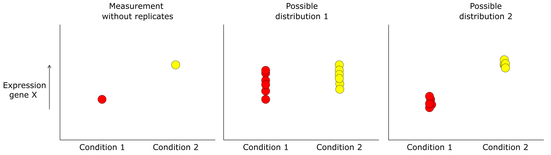
Figure 36:Difference in expression of gene X between two conditions measured without replicates and two possible distributions the measurement could have come from. Credits: CC BY-NC 4.0 Ridder et al. (2024).
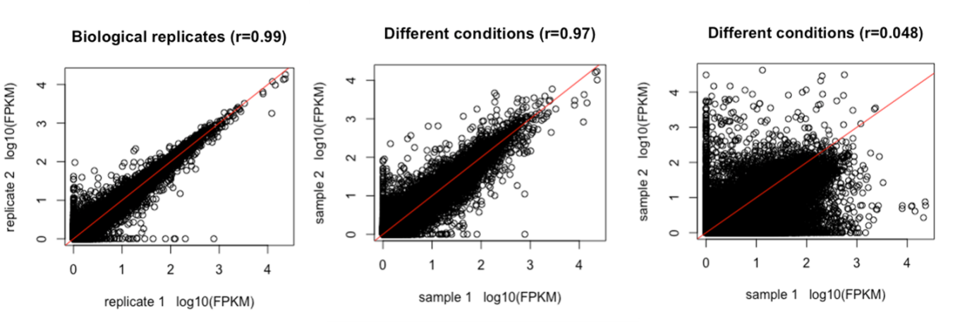
Figure 37:Comparison of FPKM values between 2 replicates (left) and two conditions (middle and right). The correlation between replicates should be very high, the differences between two conditions can be small (middle) or large (right). Credits: CC BY-NC 4.0 Ridder et al. (2024).
Visualization
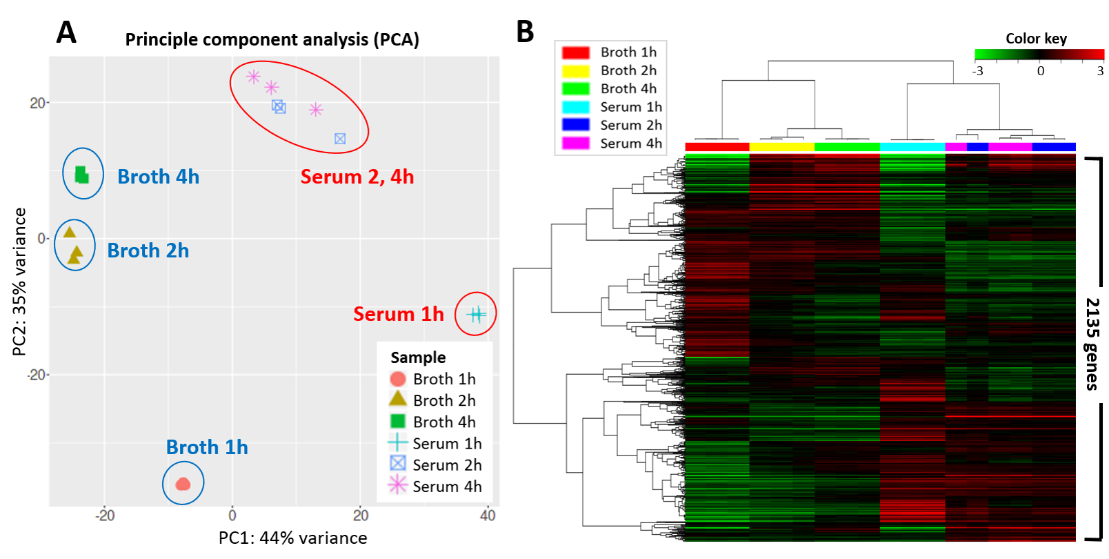
Figure 38:Visualization of the expression of 2,135 genes in Streptococcus parauberis after 1, 2, and 4 hours of growth in two different media: fish serum and broth. Each condition has been measured on 3 replicates. Left: a Principal Component Analysis (PCA) that shows there is a major separation (44% of the variance) between the two media and that there is clear progression along time. Note that there is not much expression difference after 2 and 4 hours of growth on serum. Right: a heatmap visualizes the entire dataset, with colors indicating z-score normalized expression values: green is low, black is medium and red is high expression. Rows are genes, columns indicate growth condition, both are clustered. Credits: CC BY 4.0 Lee et al. (2021).
While omics data can be inspected in, for example, Microsoft Excel, it is very hard to make sense of a data matrix with tens of thousands of genes and dozens to hundreds of samples. It is therefore wise to first use methods to visualize or summarize the data to see whether major patterns or outliers can already be detected. A widely used visualization is the so-called heatmap, an image of the matrix (genes-by-samples) where each measurement is represented by a colour. If the data is clustered along both genes and samples, interesting patterns may be easy to spot. A second approach often used in initial data exploration is Principal Component Analysis (PCA), which plots samples (or genes) along the main axes of variation in the data. If colour or markers are added, a PCA plot serves very well to detect groups and outliers. Both visualizations are illustrated in Figure 38.
Differential abundance
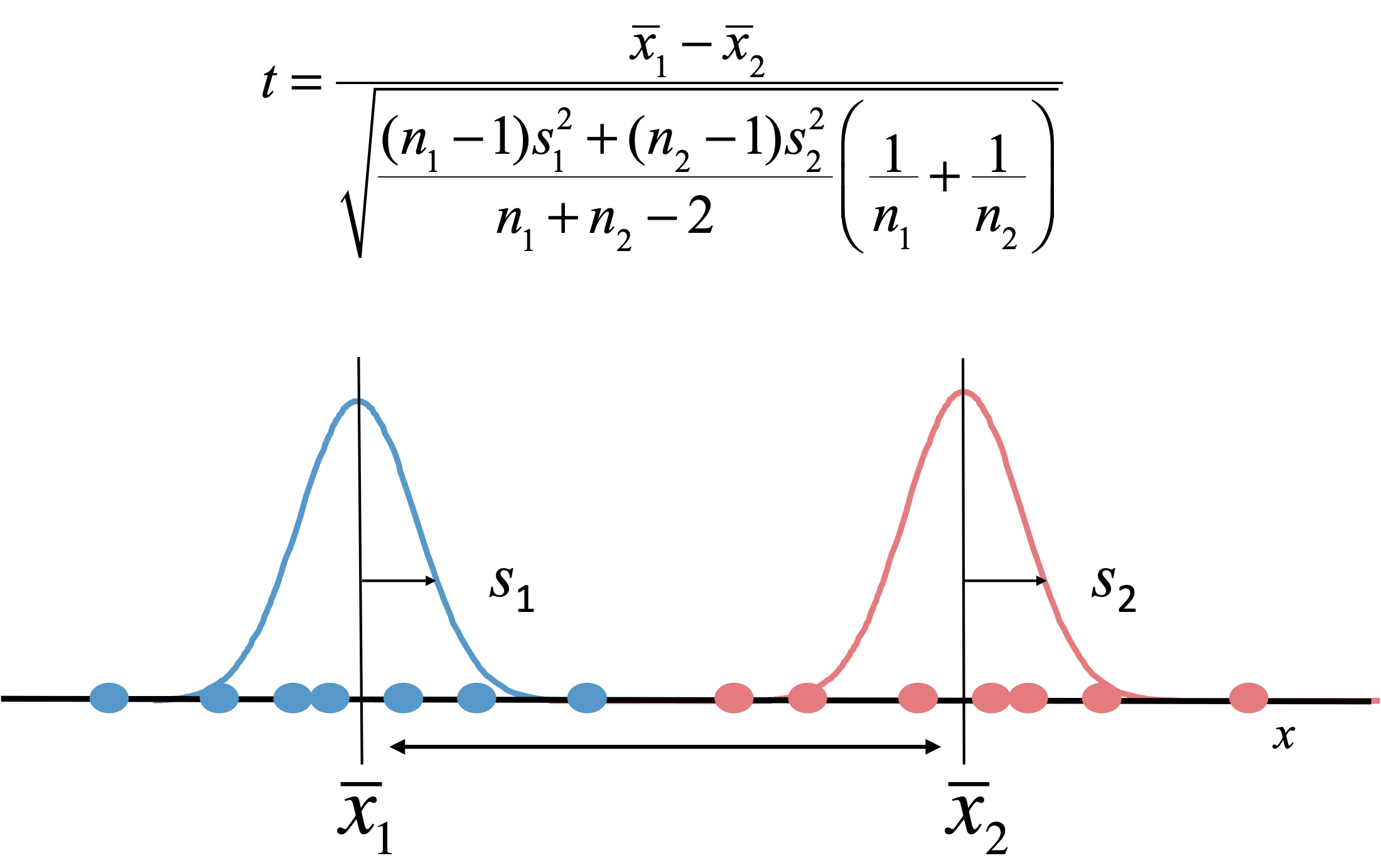
Figure 39:The simplest test for differential abundance of a gene between two conditions is the t-test. The t-statistic is a measure for the difference between the means x of two distributions, corrected by the uncertainty expressed in terms of their standard deviation s. A p-value, the probability that we find a t-statistic as large or larger by chance, can be calculated using the t-distribution. Credits: CC BY-NC 4.0 Ridder et al. (2024).
Differential abundance is the most widely used analysis on omics data. The goal is to compare abundance levels between two classes, conditions, strains, cell types, etc. - for example, healthy vs. diseased tissue, with or without a certain drug, in different growth conditions, etc. The simplest approach is to collect a number of replicate measurements under both conditions and, for each gene, perform a simple statistical test such as the t-test (Figure 39). Each test gives a p-value, and genes with a p-value below a certain threshold, say 5%, could then called significantly differentially expressed.
There are two caveats:
- If you perform an individual test for each of thousands of genes, at a threshold of 5% you would still incorrectly call many hundreds to thousands genes differentially expressed. To solve this, p-values are generally adjusted for multiple testing, i.e., made larger.
- If the variation (standard deviation s in Figure 39) is low enough, a small difference can become significant even if the actual abundance difference is small. Therefore, in many experiments an additional requirement to select genes is that the fold change is large enough. Often, this is expressed as log2(fold change), where +1 means that a gene is 2x more expressed, +2 means 4x more expressed, -1 means 2x less expressed and so on.
There are a number of similar, but more sophisticated approaches that better match with experimental follow-up, but these are out of scope for this book.
Time series analysis
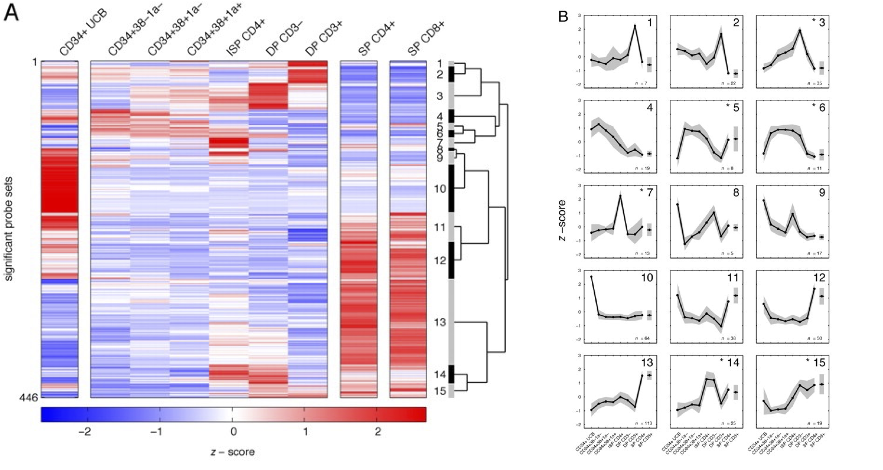
Figure 40:Transcriptomics of various stages of T-cell development, i.e., a time series analysis. Left: heatmap of the 446 genes with most variable gene expression levels, clustered into 15 clusters. Right: average expression profiles of each cluster show that different groups of genes peak in expression in different development stages. These genes may be regulated in the same way and be active in similar biological processes. Credits: CC BY-NC-SA 4.0 Dik et al. (2005).
Often it is more interesting to follow abundance over time rather than compare it at one specific timepoint, e.g., when tracking the response to a drug, a change in growth conditions, regulation of organ development, and so on. Given the cost of omics measurements, a major challenge is to select optimal time points for sampling, balancing the information obtained with the investment. Subsequent analyses include clustering to find similarly regulated genes (see below) and more advanced methods that try to identify regulatory interactions by seeing which gene increase/decrease precedes that of another (set of) gene(s). Figure 40 provides an example.
Classification
Classification is related to differential abundance analysis, in that it tries to find genes that best explain the difference between conditions. However, here the goal is actually to predict the condition of a new (additional) sample based on a limited set of gene expression levels, as accurately as possible. Applications are mainly found in medicine, such as diagnosis and prognosis, but are also used to distinguish different cell types, growth stages, etc.
Clustering
Clustering methods attempt to find groups of genes that have similar abundance profiles over all samples, or (vice versa) samples that have similar abundance profiles over all genes. We call such genes or samples co-expressed. Based on the guilt-by-association principle, correlation can be used to learn about the function of genes - “if the expression of gene A is similar to that of gene B with a certain function F, then gene A likely also has function F”. This can help identify genes involved in similar processes or pathways: co-expressed genes can be co-regulated, code for interacting proteins, etc. For samples, it can help identify for example disease subtypes, different genotypes, etc. that may be helpful to learn about different outcomes. Clustering is often used to order the rows and columns of a heatmap (as in Figure 38 and Figure 40), after which obvious clusters should become visible as large color blocks.
Enrichment
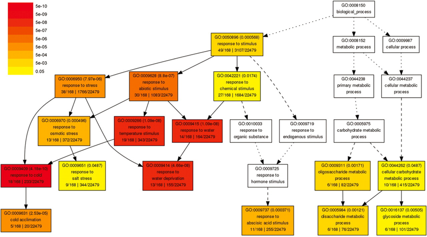
Figure 41:An example part of the Gene Ontology (GO), in the biological process category. Lower-level terms are specific instantiations of the higher-level ones. In this figure, GO terms are coloured according to the p-value in an enrichment test. Credits: CC BY-NC 4.0 Ridder et al. (2024).
A final often used analysis is enrichment, in which we use gene functional annotation to learn about a set of genes, such as a list of differentially expressed genes or a cluster. The most widely used annotation for genes is the Gene Ontology, a structured dictionary of terms that describe the molecular functions of genes and their involvement in biological processes or cellular components at different levels of detail (Figure 41). A statistical test then assesses how significantly often (more than by chance) we find a certain annotation in our list of genes. Like differential abundance, the p-values produced should be adjusted for multiple testing. The resulting significant annotations can help interpret the outcome of an experiment at a higher level than that of individual genes.
Outlook
This section on omics data analysis is likely the most prone to obsolescence. We have only touched upon or even left out recent developments in single-molecule measurements of DNA, RNA, and proteins, of single-cell and spatial omics analysis, where molecules are measured in individual cells or at grid points in tissues, and accompanying developments in deep learning that promise to provide foundation models to capitalize on the large volumes of omics data in order to learn the “language” of DNA and proteins and to solve specific tasks. The end goal, a systems biology simulation of the living cell, is still far from reality, but may be reached sooner than we now believe possible.
Practical assignments
This practical contains questions and exercises to help you process the study materials of Chapter 5. You have 2 mornings to work your way through the exercises. In a single session you should aim to get about halfway through this guide (i.e., day 1: assignment 1-3, day 2: assignment 4, 5 and project preparation exercise). Use the time indication to make sure that you do not get stuck in one assignment. These practical exercises offer you the best preparation for the project. Especially the project preparation exercise at the end is a good reflection of the level that is required to write a good project report. Make sure that you develop your practical skills now, in order to apply them during the project.
Note, the answers will be published after the practical!
Appendix: -omics measurement technology
Much of what we now know about the molecular biology of the cell is based on extensive measurements, using a range of ever improving devices. The amount of measurement data and its coverage, reliability, biases etc. crucially depend on the technology underlying these devices and its limitations. Moreover, (lack of) technology influences what we cannot yet measure and are thus relatively “blind” to. This is the most important information to keep in mind when analysing the resulting data. For this reason we limited ourselves to listing the main data characteristics in the main text. Here, we provide slightly more background on the most important (historical) technologies for the interested reader.
Genomics
Transcriptomics
Proteomics and metabolomics
Glossary
- 2nd generation sequencing
- see next-generation sequencing
- Classification
- Predicting an output of interest (e.g. a phenotype) based on -omics data.
- Clustering
- Finding groups in data sets to learn about common factors, i.e. similar diseases (when clustering samples) or similar functions (when clustering genes).
- Contig
- Part of a genome assembly, contiguous sequence that can be assembled without problems or gaps.
- Co-segration
- Which parts of the genome were inherited together from either the mother or the father.
- Deletion
- Deletion of a small number of nucleotides (<100bp) in a genome compared to the reference.
- Differential abundance analysis
- Comparison of levels between conditions, cell types, strains etc., often based on a statistical test.
- Draft genome
- Genome assembly that is the preliminary result of a genome assembly to the level of contigs, contains most genic regions, but is otherwise fragmented.
- Enrichment
- Identifying biological processes/functions that are found significantly more in a set of genes/proteins than expected by chance.
- Epigenetics
- Heritable change in gene expression that occur without changes in the genome sequence.
- Epigenomics
- Measuring the epigenetic state of the entire genome.
- Flow-cell
- Part of the sequencing device where the DNA is deposited on and the actual sequencing process happens.
- Fold change
- Relative measurement comparing two conditions, often log2-transformed for easy interpretation and visualization.
- Functional annotation
- Determine the putative function of structurally annotated genes in a genome assembly using homology methods.
- Functional genomics
- Field of study on gene/protein functions and interactions.
- Functional proteomics
- Measurements of interactions between proteins and other proteins, DNA etc.
- Heatmap
- A visual representation of a data matrix as an image, where cell colors reflect values. Often clustered along one or both axes to help identify groups of samples/genes with similar expression levels.
- High-throughput
- Technology to collect large amounts of measurement data without the need for extensive human intervention.
- Hybridisation
- Successful mating between individuals of two different, but closely related species, that generated offspring.
- Insertion
- Insertion of a small number of nucleotides (<100bp) in a genome compared to the reference.
- Introgression
- Parts of a genome that originate from a different species. The result of hybridisation of the two species at some point in the past.
- Mapping
- Finding locations in the genome that (nearly, allowing for errors) match a given short DNA sequence, such as a sequencing read.
- Mass spectrometry (MS)
- Measurement technology for molecule weight, based on ionization, separation and detection.
- Metabolomics
- Measurements of the presence or levels of metabolites in a cell.
- Microarrays
- Devices that measure gene expression based on fluorescence of complementary DNA sequences binding to DNA attached to specific spots on a surface. Superseded by RNAseq, but still widely found in databases.
- MNP
- Multiple nucleotide polymorphism, change of a number of adjacent nucleotides in a genome compared to the reference.
- M/z
- Unit of measurement of mass spectrometry devices: mass-over-charge ratio.
- Next-generation sequencing
- NGS, also 2nd generation sequencing; Sequencing technologies post Sanger sequencing, mostly refers to Illumina sequencing.
- Omics
- Studying the totality of something; for example, the expression of all genes (transcriptomics).
- Paired-end read
- In Illumina sequence, two reads that come from the same fragment of DNA: the first sequenced from one end, and the second in reverse complement from the other end. When the original DNA fragment was longer than the two reads, there is a gap between the two reads when aligned to the reference.
- Phenomics
- Measurements on macroscopic phenotypes (traits) of tissues and organisms.
- Principal Component Analysis (PCA)
- Projection of data with many measurements onto the directions which retain as much variation as possible. Often used for projecting onto 2 dimensions in order to visually analyze a given data set.
- Proteomics
- Measurements on proteins in a cell.
- Quantitative proteomics
- Measurements presence/absence or levels of proteins in a cell.
- Q-score
- Quality score, used to indicate quality of a base in sequencing, or variant in case of variant calling.
- Repeat region
- DNA sequence that is repeated many times across a genome. Copies might vary slightly between each other.
- RNAseq
- Transcriptomics measurements by DNA sequencing technology, after converting RNA to cDNA.
- Shotgun proteomics
- Measuring protein levels by MS after fragmenting into peptides at known cleavage sites, then look up the peptides in protein sequ
- Spliced mapping / spliced alignment
- Mapping of RNAseq reads, taking into account that introns are not present in transcripts and that reads therefore can partly map to two nearby locations.
- Split reads
- Reads that are split into two parts during sequence algnment, with both parts aligning to different sections of the reference. See also Spliced alignment.
- Structural annotation
- Determining the location and features of (protein coding) genes in a genome assembly
- Systems biology
- An approach to studying complex biological systems holistically, by constructing and iteratively updating models.
- Telomere-to-telomere assembly
- T2T; genome assembly that covers all sequence of an organism, whithout gaps, assembled to each chromosome from one telomere to the other.
- t-test
- Widely used statistical test for difference between means of two distributions. It assumes that data is normally distributed, which in practice is often not the case so more sophisticated tests are used.
- Time series analysis
- Analysing measurements taken over time, to study changes.
- Transcript quantification
- Conversion and normalisation (for gene length, library size etc.) of RNAseq read counts for further analysis.
- Transcriptomics
- Measurements of the expression levels of all genes in a cell.
- Whole genome shotgun sequencing
- WGS. Sequencing of all parts of a genome simultaniously whithout a priory knowing which part is which.
- Ridder, D. de, Kupczok, A., Holmer, R., Bakker, F., Hooft, J. van der, Risse, J., Navarro, J., & Sardjoe, T. (2024). Self-created figure.
- Narayanese. (2008). Centraldogma nodetails. https://commons.wikimedia.org/w/index.php?curid=36890617
- Darryl Leja, N. (2003). Human Genome Project Timeline. https://commons.wikimedia.org/wiki/File:Human_Genome_Project_Timeline_(26964377742).jpg
- Abizar. (2010). Genome Sizes. https://commons.wikimedia.org/w/index.php?curid=19537795
- Ehamberg. (2011). Haploid, diploid ,triploid and tetraploid. https://commons.wikimedia.org/w/index.php?curid=13308417
- Nederbragt, L. (2016). developments in NGS. 10.6084/m9.figshare.100940.v9
- Ockerbloom, M. M. (2020). MinION Portable Gene Sequencer. https://commons.wikimedia.org/wiki/File:MinION_Portable_Gene_Sequencer_IMG_20200219_170422318.jpg
- Ashari, K. S., Roslan, N. S., Omar, A. R., Bejo, M. H., Ideris, A., & Mat Isa, N. (2019). Genome sequencing and analysis of Salmonella enterica subsp. enterica serovar Stanley UPM 517: Insights on its virulence-associated elements and their potentials as vaccine candidates. PeerJ, 7, e6948. 10.7717/peerj.6948
- Murayama, H. (1919). Three squirrel fish swimming in the sea. https://wellcomecollection.org/works/sxqzrw76/images?id=erq548bv
- Kleinjan, D. A., Seawright, A., Mella, S., Carr, C. B., Tyas, D. A., Simpson, T. I., Mason, J. O., Price, D. J., & van Heyningen, V. (2006). Long-range downstream enhancers are essential for Pax6 expression. Developmental Biology, 299(2), 563–581. https://doi.org/10.1016/j.ydbio.2006.08.060
- Nurk, S., Koren, S., Rhie, A., Rautiainen, M., Bzikadze, A. V., Mikheenko, A., Vollger, M. R., Altemose, N., Uralsky, L., Gershman, A., Aganezov, S., Hoyt, S. J., Diekhans, M., Logsdon, G. A., Alonge, M., Antonarakis, S. E., Borchers, M., Bouffard, G. G., Brooks, S. Y., … Phillippy, A. M. (2022). The complete sequence of a human genome. Science, 376(6588), 44–53. 10.1126/science.abj6987
- Ausmus, S. (2006). Carrots of many colors. https://commons.m.wikimedia.org/wiki/File:Carrots_of_many_colors.jpg
- Hellens, R. P., Moreau, C., Lin-Wang, K., Schwinn, K. E., Thomson, S. J., Fiers, M. W. E. J., Frew, T. J., Murray, S. R., Hofer, J. M. I., Jacobs, J. M. E., Davies, K. M., Allan, A. C., Bendahmane, A., Coyne, C. J., Timmerman-Vaughan, G. M., & Noel Ellis, T. H. (2010). Identification of Mendel’s White Flower Character. PLOS ONE. 10.1371/journal.pone.0013230
- Yengo, L., Vedantam, S., Marouli, E., Sidorenko, J., Bartell, E., Sakaue, S., Graff, M., Eliasen, A. U., Jiang, Y., Raghavan, S., Miao, J., Arias, J. D., Graham, S. E., Mukamel, R. E., Spracklen, C. N., Yin, X., Chen, S.-H., Ferreira, T., Highland, H. H., … Hirschhorn, J. N. (2022). A saturated map of common genetic variants associated with human height. Nature, 610(7933), 704–712. 10.1038/s41586-022-05275-y
- Mylavarapu, S., Das, A., & Roy, M. (2018). Role of BRCA Mutations in the Modulation of Response to Platinum Therapy. Frontiers in Oncology, 8. 10.3389/fonc.2018.00016