📘 This content is part of version: v1.0.0 (Major release)In this chapter you will learn what phylogenetic trees are, how you can interpret these trees, and how you can infer them from multiple sequence alignments of either DNA or amino acid sequences.
Introduction
In this chapter you will learn to use a Multiple Sequence Alignment (MSA), like the ones you compiled in chapter 2, and visualize the variation it contains as a phylogenetic tree. A phylogenetic tree is considered a highly efficient data structure summarizing the data and its variation contained in your MSA. A tree is built from characters which are the individual columns or positions in your MSA. Characters have states, which are in this case the individual nucleotide or amino acid substitutions occurring in that position (see characters & trees below). Invariable characters are columns or positions ‘occupied’ by just one type of nucleotide or amino acid, whereas variable characters may have up to 4 different nucleotides or up to 20 amino acids per position.
DNA and amino acid (AA) sequences contain the information necessary for building protein structure. Comparing them in an MSA will enable insight how these structures, and their associated functions, may have changed over evolutionary times since they descended from an ancestral sequence. The more character state changes (i.e., substitutions) occur between sequences, the more diverged they are and probably also less related (see related, diverged below), and hence the further apart they will occur on your phylogenetic tree. The information contained in your tree is hierarchical in nature, meaning that it is built-up as nested sets of subtrees that are also known as clades. A clade is a group containing an ancestor together with all its descendants and is also referred to as a monophyletic group.
Rationale
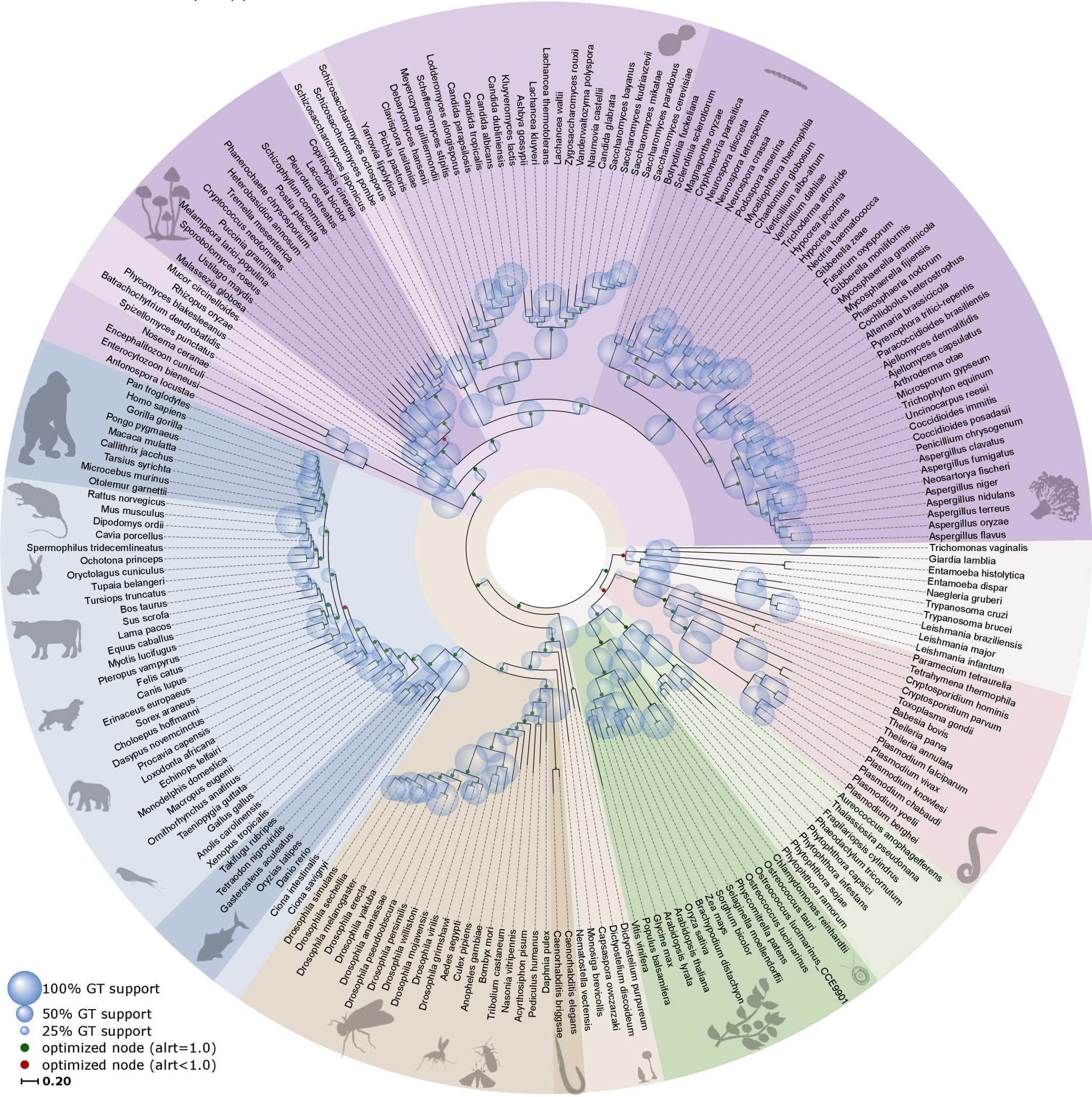
Figure 1:Simplified Tree of Life. Credits: CC BY 4.0 Huerta-Cepas et al. (2014).
Why should we study Phylogenetics and what is it about? Ever since Darwin we know that all living things are connected in a tapestry of life, forming a phylogenetic tree of everything (Figure 1). Phylogenetics aims at understanding evolutionary relationships among genes, species, and higher taxa and as such it is relevant to almost all biological questions. Why? Because an evolutionary context (rather than a ‘snapshot’ perspective) allows identifying evolutionary lineages and their origins, and can provide information on how lifeforms and sequences change and adapt across millions of years. Examples are studying the evolution of gene families within genomes, or the build-up of species relationships in a lineage.
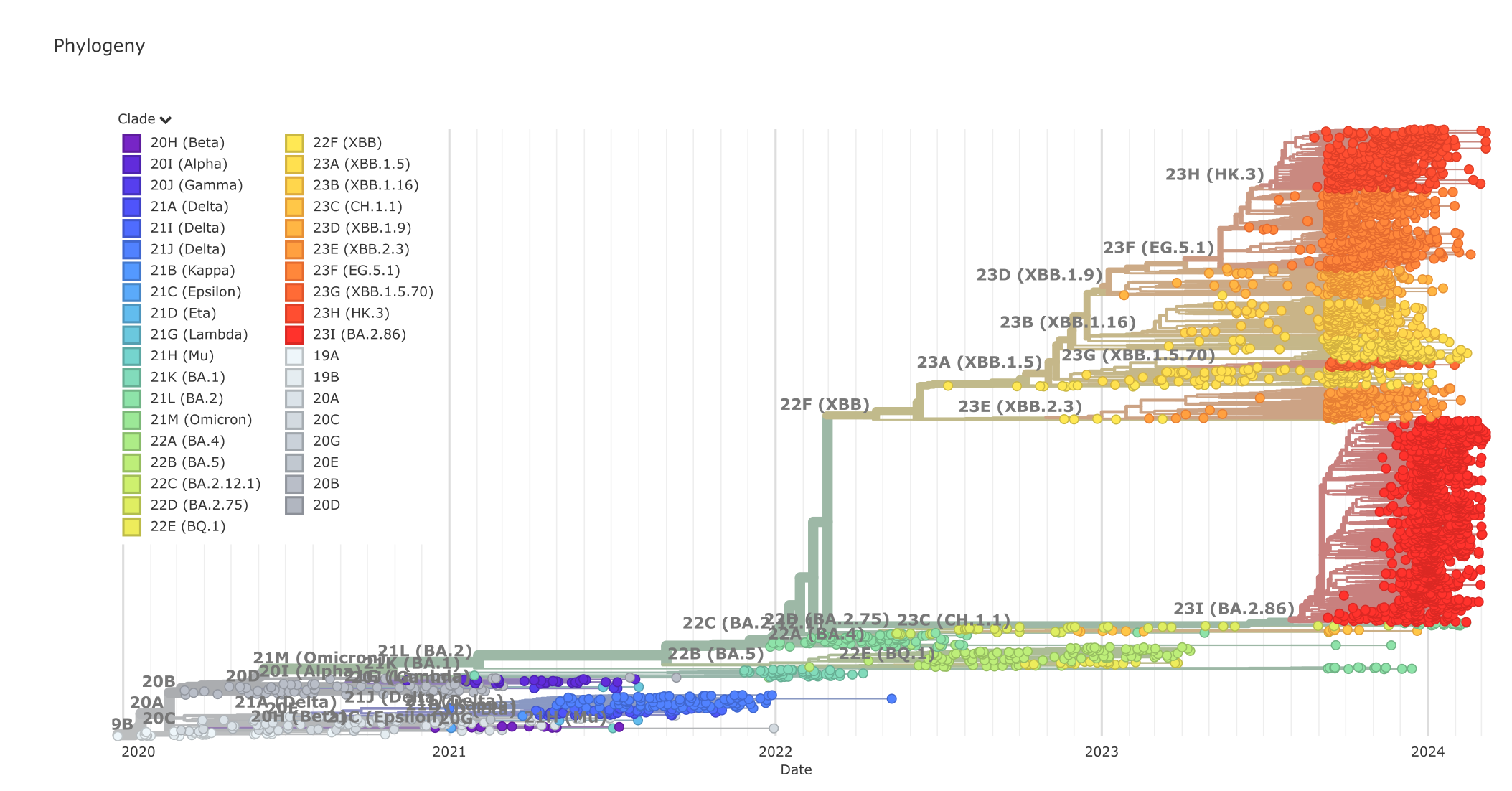
Figure 2:The SARS-CoV-2 phylogenetic tree, March 2024. Credits: CC BY 4.0 Hadfield et al. (2018).
Other examples are studying Covid-19 and other pathogen outbreaks (Figure 2), studying molecular evolution and the accumulation of substitutions in a multiple sequence alignment (MSA). Or, studying population history within a species, reconstructing historical biogeography: In all these cases having an accurate phylogenetic tree is crucial, because we want to be able to reconstruct evolutionary lineages (the branches in phylogenetic trees) and how they evolved, changed, duplicated, or went extinct. By accurate we mean estimating relationships that are as close as possible to the actual (historic) relationships, which we cannot know for sure. As they happened in the past we cannot prove them, but they are hypotheses (of relationships) that we can only corroborate (confirm, seek support for).
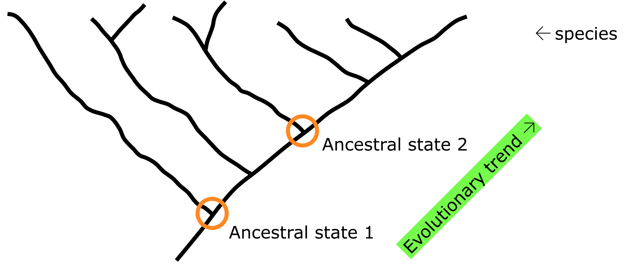
Figure 3:Comparing species (or genes) in a phylogenetic tree allows inference of ancestral states and evolutionary trends. Credits: CC BY-NC 4.0 Ridder et al. (2024).
When a phylogenetic tree is known for a specific group, and it is properly Rooted, the ancestral States for its Characters can in principle be reconstructed (for instance the ancestral amino acid residues in a protein sequence) for each node in the tree. With that, evolutionary trends (towards current conditions) can be inferred, enabling the study of character evolution, i.e., how things change over time (Figure 3).
Phylogenetic trees: structure & interpretation
Like all trees, phylogenetic trees come with a stem, branches, leaves and ideally a root. What makes phylogenetic trees special however is that they are actually hypotheses of evolutionary relationships, as outlined in the previous section. The leaves or external nodes are then the individuals (or sequences) that are observed and compared, which are also referred to as operational taxonomic units (OTUs) or terminals. The branches and nodes are the lineages or clades that are inferred, i.e., not observed. A Clade is an ancestral node together with all its descendants, which is also referred to as a monophyletic group, an example of Monophyly. They are recognised by the horizontal lines connecting the OTUs and HTUs (hypothetical taxonomic units) in your phylogenetic tree, as for instance shown in Figure 4.
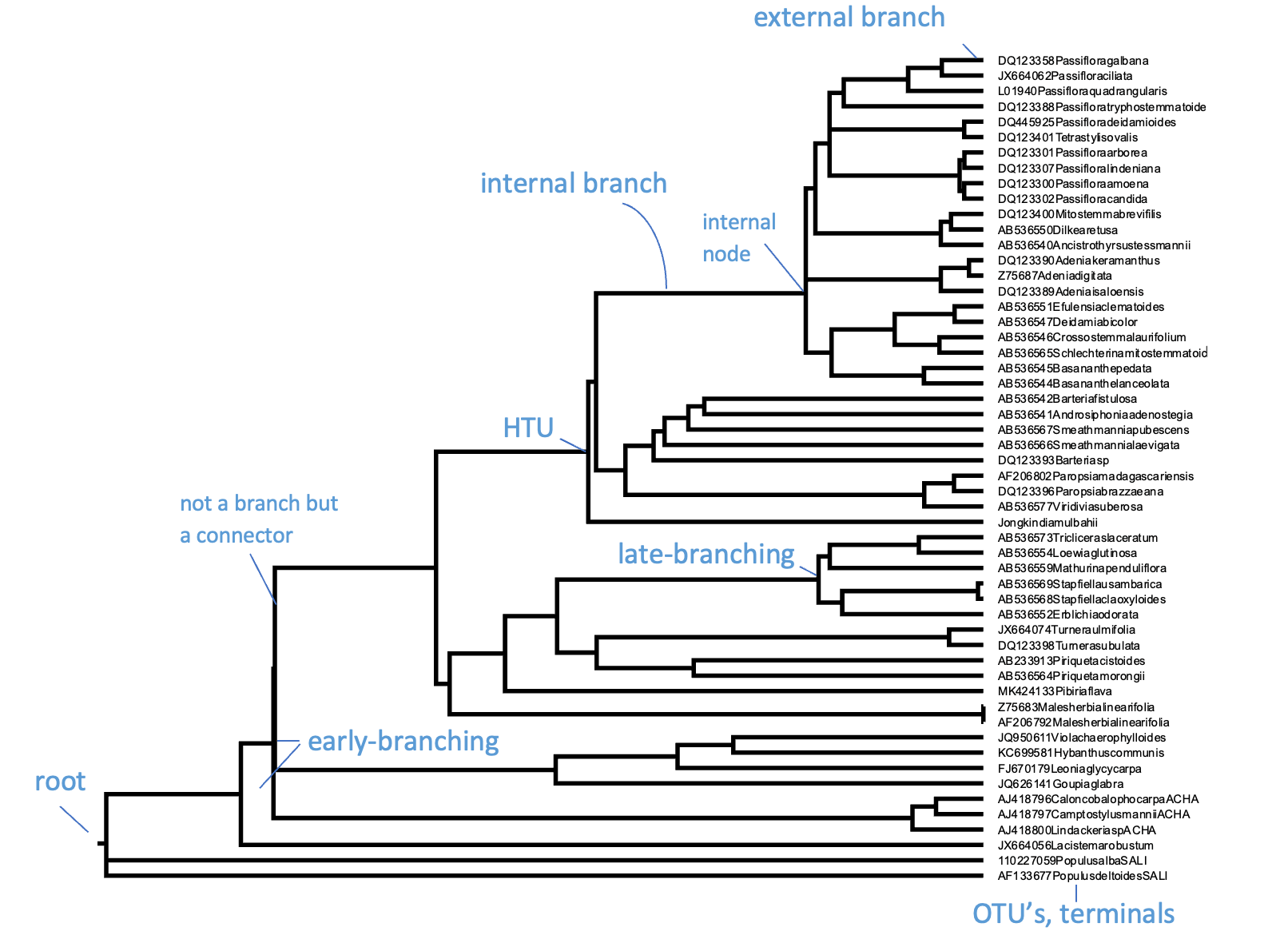
Figure 4:A rooted ultrametric phylogenetic tree with its main parts and characteristics indicated. Here, the OTUs are GenBank plant chloroplast gene accessions, the names of which have been condensed. Credits: CC BY-NC 4.0 Ridder et al. (2024).
Whereas the horizontal lines represent the actual branches, the vertical lines do not have a meaning and are just there to connect the branches and clades; they will get longer when more terminals are included but do not have a relation with the data (i.e., the MSA). Branches are connected via nodes, that can be internal (HTUs) or external (OTUs). Internal nodes represent hypothetical ancestors that are not observed or sequenced but inferred or reconstructed. As outlined above, external nodes are the actual individuals observed; they are never connected directly to each other, only through internal nodes. These individuals can represent genes, species or higher taxa, but they are never categories (or averages), as characters and states are indivisible observations scored on individuals. Branches and nodes collectively build the Tree topology, i.e., the structure of the tree.
One of the most important aspects of a phylogenetic tree is whether it is rooted, meaning whether we can distinguish which nodes are old and which are more recent, and also what clades are present. Rooting is done by selecting an Outgroup, which is a reference taxon outside the group of interest (this is described in more detail in section Rooting & clades). It is important to realise that most phylogenetic reconstruction methods actually produce unrooted trees, which can then rooted using an outgroup to visualize in what direction evolution proceeded and which clades can be identified.
Related, diverged
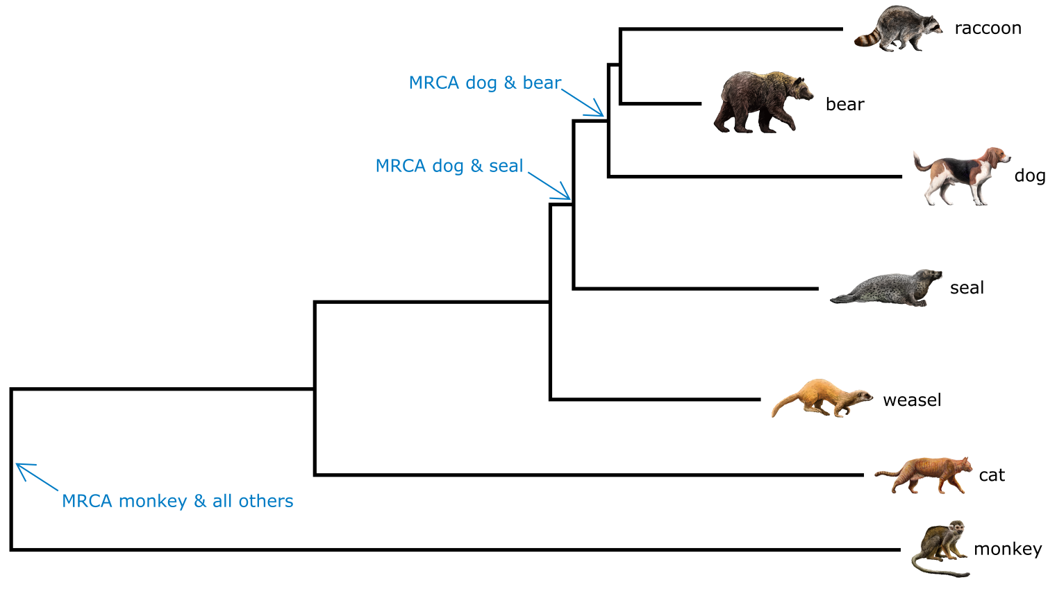
Figure 5:Additive phylogenetic tree of mammalian species, rooted on monkey. The MRCA of monkey, bear, seal and dog is indicated. Tree topology informs relatedness, branch lengths correspond to divergence. Credits: CC BY-NC 4.0 Ridder et al. (2024). Made using imagery from: CC BY 4.0 DataBase Center for Life Science (DBCLS) (2023)
In a rooted phylogenetic tree, terminals sharing a more recent common ancestor are more closely related than terminals sharing a less recent common ancestor. Thus, in Figure 5, dog and bear are more related than dog and seal, because dog and bear share a more recent common ancestor. On the other hand, monkey and dog are as related as monkey and cat, because they all share the same most recent common ancestor (MRCA). Being unrelated is not the same as being diverged, as divergence means the amount of change accumulated since the split of two lineages, which is reflected in the Branch lengths (or in distances). In our example, raccoon and dog would be more diverged than raccoon and bear, but not more closely related.
Cladogram, additive and ultrametric
Phylogenetic trees come in three flavors: Ultrametric trees_, Additive trees, and Cladograms. When all paths starting from the root to each external node are of equal length, you could interpret the length of a path through the tree as proportional to time and thus equally old as other paths; the ages of nodes can then in principle be inferred. Such a tree is known as an ultrametric tree, which can be easily recognised by its topology in which all terminal branches line up, usually to the right. Another, more common type of phylogenetic tree is the additive tree, in which branch lengths are proportional not to time but to the amount of change occurring in your data set (the MSA). Therefore, the more changes (i.e., substitutions, insertions, deletions) occur for an individual, the longer the branch to its MRCA will be in the additive tree. Most phylogenetic and tree building platforms or software packages produce additive trees. Producing ultrametric trees usually requires taking extra steps, with each step introducing uncertainty. You could argue that ultrametric trees are one extra step away from the data compared to additive trees. Only when the data accumulates substitutions in a strictly clock-like manner (i.e., like radio-active decay) would the ultrametric and additive tree version be the same. However, such strict molecular clocks are never encountered in real data. Finally, a cladogram-style tree is a ‘schematic tree’ meant to only show the topology of your tree. It therefore has artificial (equal) branch lengths, including for terminal branches.
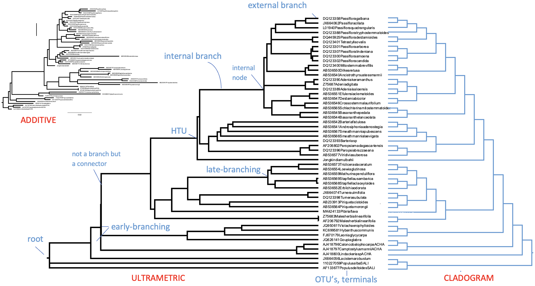
Figure 6:A rooted phylogenetic tree with its main parts and characteristics indicated. Here, the OTUs are GenBank plant chloroplast gene accessions, the names of which have been condensed. For the same data, the tree is given as additive tree (top) and as an ultrametric tree (bottom left) with branch lengths corresponding to time. On the right, flipped, the same tree as cladogram, with branch lengths only indicating the structure of the trees. Credits: CC BY-NC 4.0 Ridder et al. (2024)
Tree resolution
The resolution of a phylogenetic tree is the extent to which nodes and branches (clades) can be inferred/observed from the tree. Trees can be fully resolved, in which case each internal node is connected to three branches: the ancestral branch and two subtending branches. Such trees are called bi-furcating or dichotomous, meaning that each branch splits into two and there are no uncertainties on branching order or resolution of nodes. Frequently however, phylogenetic trees will be partly resolved and contain Polytomies, which are nodes connected to (many) more than three branches. Polytomies represent parts of the phylogenetic tree that are uncertain in terms of branching order of the lineages involved. This can be due to there being insufficient information in the MSA for resolving the lineages, or ample but conflicting signal. Polytomies are usually interpreted as soft, meaning that the data used does not allow to resolve the lineages inferred (Figure 7).
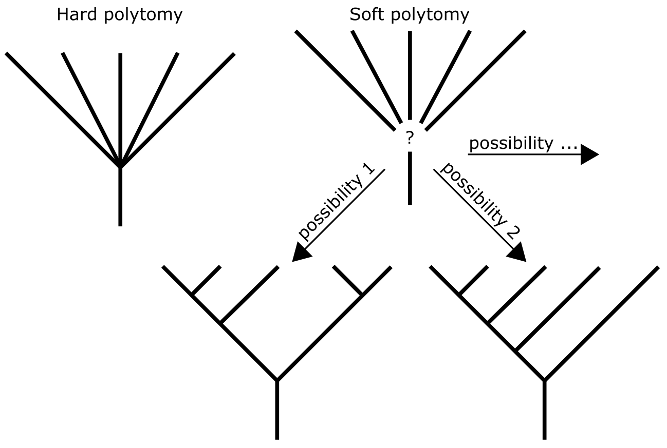
Figure 7:Hard and soft polytomies in a phylogenetic tree. The soft polytomy can imply different tree resolutions. Credits: CC BY-NC 4.0 Ridder et al. (2024).
In contrast, the hard interpretation would be: instantaneous speciation, i.e., an ancestral species lineage split up so fast that the new lineages do not have sufficient unique substitutions to ‘mark’ them and to assign them an internal node in the tree. An example is the late-Tertiary radiation of mammalian orders, after the fairly quick establishment of cold water around the Earth’s poles, combined with that of the hot tropics. Several published mammalian phylogenetic trees contain unresolved spines or backbones.
On the other hand, gene trees (used for studying gene families) may also contain polytomies and they are usually considered as soft (the data is not decisive enough to infer a branching order). Whole genome duplications (auto-polyploidisations) are fairly well known, especially in the evolution of flowering plants. Following such an event, pairs of genes can be expected to form instantaneously, i.e., without accumulating unique substitutions, and may result in hard polytomies in gene trees.
Orthologs & paralogs
When the terminals included are actually gene or protein sequences, the tree will be a Gene tree, likely containing homologs (derived from a common ancestor gene), possibly also orthologs and paralogs. Orthology is the occurrence of corresponding, homologous (and mostly similar), genes in lineages resulting from speciation. For instance, human beta globin and chimp beta globin are orthologs. Usually, these genes will have the same function in different species, but this doesn’t necessarily have to be the case. In contrast, paralogy is the occurrence of similar genes resulting not from speciation but from Gene duplication. For example, proteins from a gene family with different functions in the same species. Such similar genes are referred to as paralogs, which are visualized as multiple occurences of particular terminals on the tree. Figure 8A and B illustrates the process of gene duplication followed by speciation, resulting in two parallel subtrees (the blue X tree and the green X’ tree). Figure 8C shows the challenge with using both orthologs and paralogs in phylogenetic analysis when not all members of a gene family have been sampled.
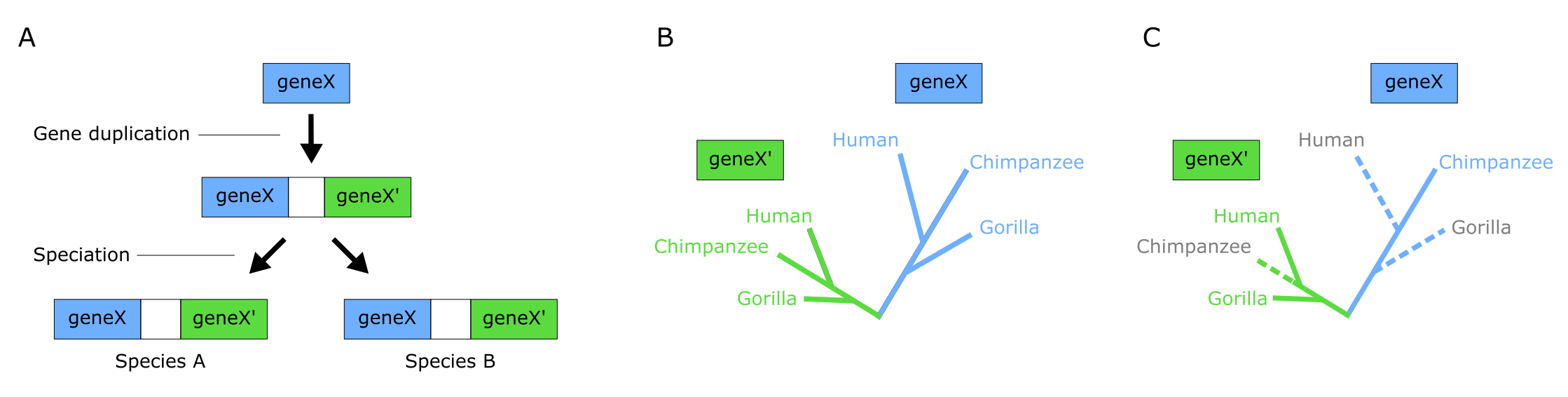
Figure 8:The challenge of paralogs: (A) Paralogous genes are created by gene duplication events. Gene X is duplicated in a (recent) common ancestor (RCA) of species A and B resulting in paralogous genes X and X’. Species A and B inherit both copies of the gene (unless one or the other is lost somewhere along the way). (B) Phylogenetic analysis of the X/X’ gene family gives two parallel phylogenies. All sequences of gene X are orthologues of each other, as are all sequences of gene X’. However, X and X’ are paralogues. Both the X and X’ subtrees show the true relationships among the three species. The subtrees are also each other’s natural outgroup, and as a result each subtree is rooted with the other (reciprocally rooting). (C ) A tree of the X/X’ gene family can be misleading if not all the sequences are included (because of incomplete sampling or Gene loss). If the broken branches are missing, then the true species relationships are misrepresented. Credits: CC BY-NC 4.0 Ridder et al. (2024).
In Figure 9, a sequence of events is given involving two duplications and one speciation event that can lead to a set of homologous genes in two species. Some of these are orthologs and some are paralogs that have acquired new functions. A Species tree is depicted by the pale blue cylinders, with the branch points (nodes) in the cylinders representing speciation events. In the ancestral species (on top) a gene is present as a single copy and has function α (blue). After some time, a gene duplication event occurs within the genome, producing two identical gene copies, one of which subsequently evolves a different function, identified as β (red). As a result, α and β are now paralogous genes. Later on, a speciation event occurs resulting in two species (A and B), both containing genes α and β. Gene Bα (in species B) subsequently undergoes another duplication event, resulting in the paralogous genes Bα and Bγ. After further divergent evolution, Bγ, aquires a new function γ (green). The Bα gene is still functionally very similar to the original gene α. At the end of this period of evolution, all five genes in the two species are homologous, with three orthologous pairs: Aβ/Bβ, Aα/Bα, and Aα/Bγ. The Bα and Bγ genes are paralogous, as are any other combinations except the orthologous pairs. Note that Aα and Bγ are orthologs despite their different functions. The gene tree inferred from these five genes has multiple occurrences of both species A and B (Figure 9B).
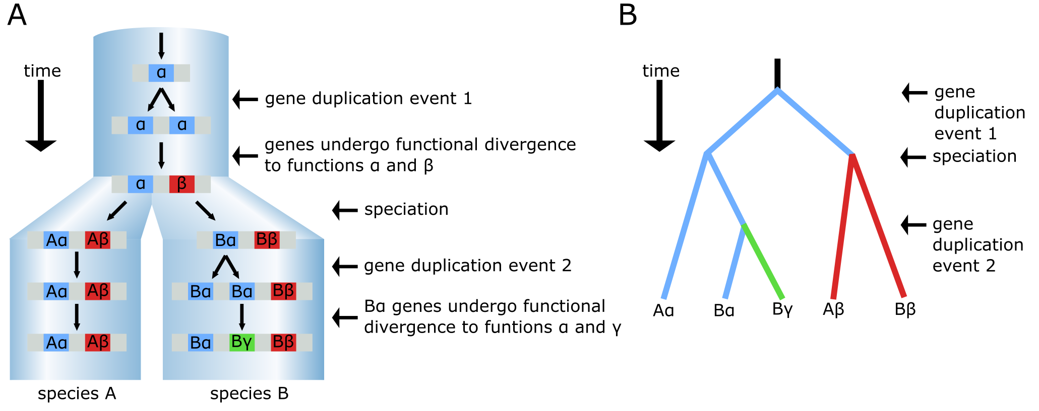
Figure 9:The evolutionary history of a gene that has undergone two separate duplication events. (A) The species tree (large blue cylinders) comprising species A and B and with indicated gene duplication and neo-functionalisation events leading to β and γ functions. (B) The phylogenetic tree that would be drawn for the resulting 5 genes in (A), here drawn as a cladogram. Credits: CC BY-NC 4.0 Ridder et al. (2024).
For another example of a gene versus species tree consider the trees in Figure 10, which are based on the comparison of Interleukin gene sequences. There are multiple occurrences of the terminals from the species tree (bovine, sheep, pig etc.) in the gene tree, each grouped with a different Interleukin sequence type. These are the paralogs, that probably resulted from gene duplication events during the proliferation of the IL clade.
Given that there are four copies of IL1 in humans (indicated with green boxes in the gene tree in Figure 10), there must have been at least three gene duplications in the history of the interleukins. Three of them are inferred from the presence of multiple copies of IL in the same mammalian species, i.e. i) in the ancestor of the IL-1α + β clade, ii) in the ancestor of the IL-1rα + β clade, and iii) as a sister pair in the IL-1β clade. Duplication δ3 is required to explain the incongruence between the mammalian species tree and the IL-1β phylogeny. The incongruence is that in the gene tree human and mouse are more closely related than either is to bovine/sheep. The species tree however indicates human to be more closely related to bovine/sheep than to mouse. In order to resolve (reconcile) this, δ3 is suggested as indicated in Figure 11.
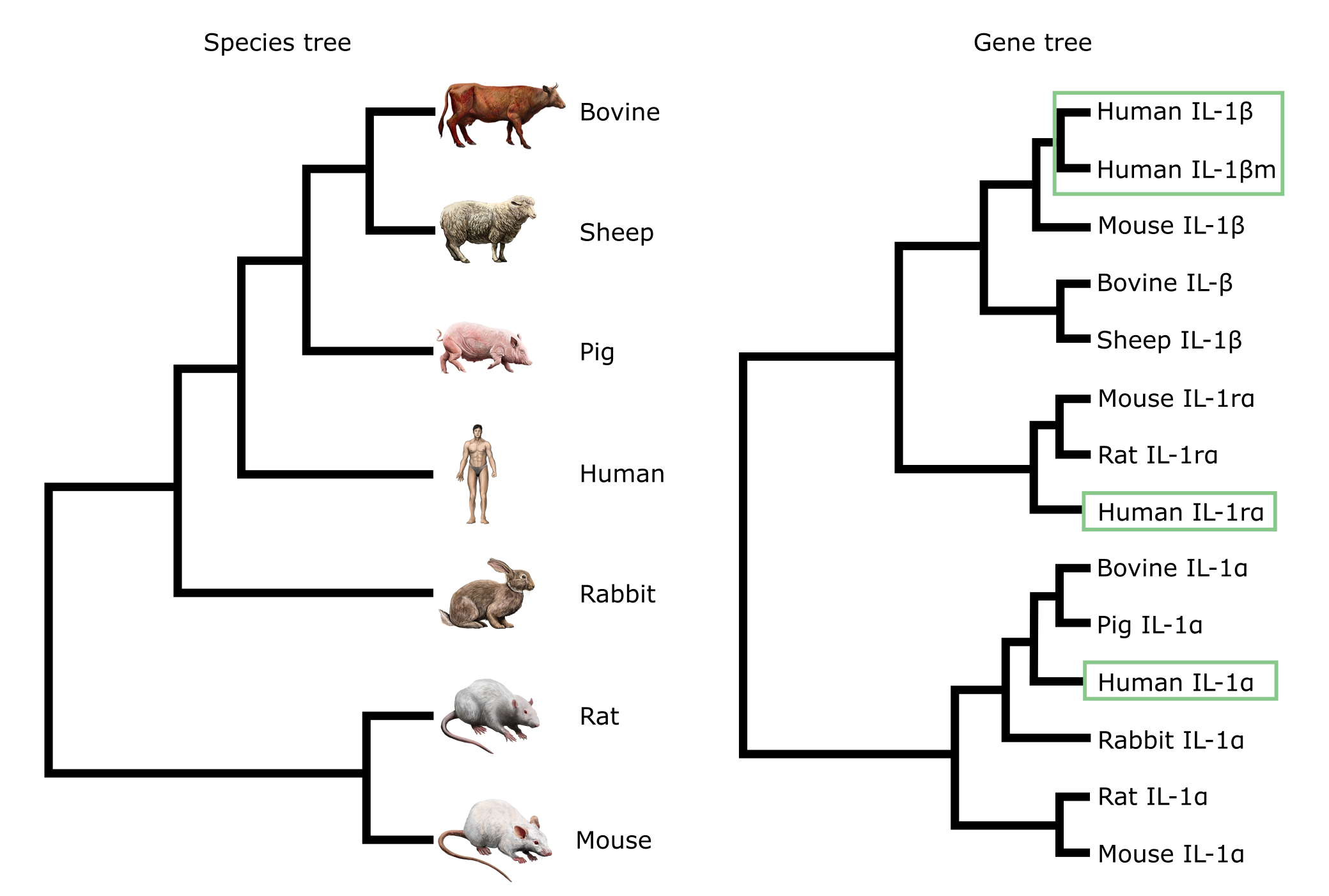
Figure 10:A species tree based on external evidence (left) and a gene tree based on a comparison of mammalian Interleukin-1 genes (right). In the gene tree, both alpha and beta copies can be seen, which are probably the result of gene duplications (see Figure 9). Occurrences of ‘Human’ in the gene tree are indicated with green boxes. Credits: CC BY-NC 4.0 Ridder et al. (2024). Made using imagery from: CC BY 4.0 DataBase Center for Life Science (DBCLS) (2021).
The tree in Figure 11 is a so-called Reconciled tree, which has been inferred as an extended tree that would be necessary to assume in order to explain the position and distribution of all IL sequence types in the gene tree. Apart from four gene duplications (marked δ1, δ2, δ3 and δ4), several gene losses (indicated with light grey branches) too would need to be assumed to explain the pattern in the gene tree in Figure 10.
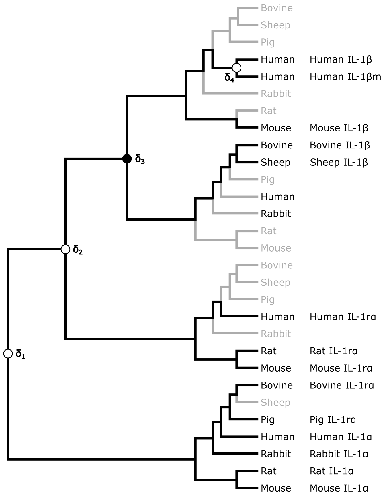
Figure 11:Reconciled tree for the mammalian interleukin-1 gene tree shown in Figure 10. Gene losses are indicated in light grey. Of the four duplications required, three are supported by the presence of multiple copies of IL in the same mammal species, and one (δ3) is required to explain the incongruence between IL-1 and mammalian phylogeny. Credits: CC BY-NC 4.0 Ridder et al. (2024).
Nodal support in phylogenetic trees: the bootstrap
Not all parts of a phylogenetic tree will be equally well-supported or strong, as defined by our character data (MSA). There can be considerable uncertainty around the estimated nodes of our tree, affecting the confidence we have in those nodes. In experimental science, usually some statistic measure is used to quantify uncertainty, for instance the mean and standard deviation of outcomes of repeated experiments. Phylogenetics, however, is not experimental but rather seeks to reconstruct historic patterns that were driven/shaped by evolution. As outlined at the beginning of this chapter, the implication is that we cannot prove phylogenies, nor repeat them, or even know whether we reconstructed the correct one. We ‘only’ have our phylogenetic trees as estimates of the true phylogeny.
In order to measure Nodal support in our phylogenetic tree, rather than producing several replicates of our MSA (which will most likely all be identical), we can draw random samples from the MSA and use these pseudo-replicate data sets to build trees (Figure 13). Repeating this process many times (hundreds or thousands) and summarizing the variation among the trees thus reconstructed, provides insight in the structure of our data and how it supports the nodes in a tree. It actually measures the sampling variance about the estimate of the phylogeny Figure 13B. This process is called Bootstrap analysis_ and will be further discussed in Maximum likelihood tree building, after we have covered the characters underlying our trees in the next section.
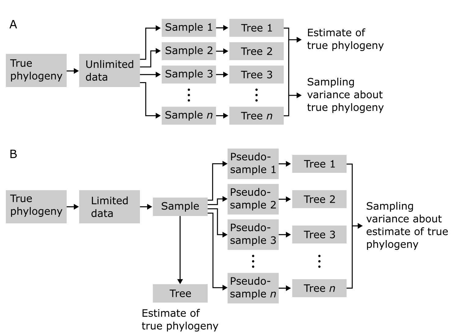
Figure 13:Bootstrap resampling analysis in phylogeny reconstruction. In case of unlimited data (A), not realistic, a summary of sample-based trees yields sampling variance about the true phylogeny. In case of limited data (B), realistic, only pseudo-samples are available, that summarise sampling variance about the estimate of true phylogeny. Credits: CC BY-NC 4.0 Ridder et al. (2024).
Characters & trees
As outlined above, phylogenetic trees are not directly observed but inferred, and represent hypotheses of evolutionary relationship, grouping individuals on the basis of shared history. The data used for comparison are the homologous sites among a set of sequences (amino acid or nucleotide) that have been aligned in an MSA in which substitutions are made visible. Homologous here means that there are corresponding positions in a gene sequence that are due to common ancestry. So, for instance, position 423 in a gene sequence from one species is homologous with position 423 in that of another species, because both species shared a recent common ancestor and we assume the genes to be orthologs. Each such position is considered a character with states that are efficiently visualized in an MSA as substitutions or ‘steps’ on the tree (Figure 14A). All nucleotide or amino acid substitutions in the MSA, both unique ones (occurring in only a single individual or sequence) and shared ones (occurring in at least two sequences), are used to build the phylogenetic tree. Invariant characters however, showing no substitutions, are not expected to contribute to the tree building process as they do not contain comparative signal. Shared substitutions are informative for building the branches of your tree, as they group terminals and hence add to the length of internal branches. Unique substitutions on the other hand only contribute to the twigs or external branch lengths and have no grouping power. The more shared substitutions occur for a set of sequences in your MSA, the stronger the resulting node in the phylogenetic tree will be supported.
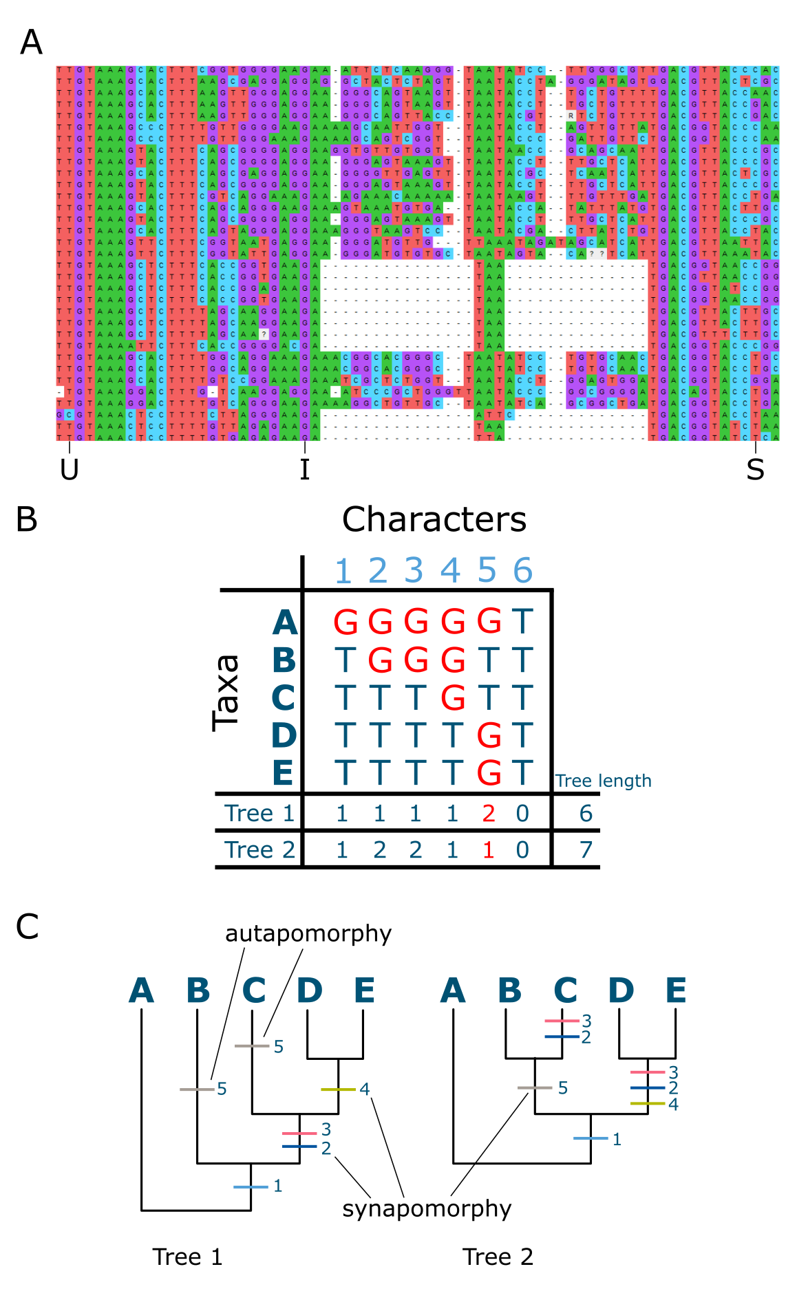
Figure 14:Characters and trees. A: Multiple sequence alignment (MSA, nucleotides) with examples of shared-derived (S), unique (U) as well as invariant (I) characters indicated; B: MSA containing S, U and I characters and the number of steps per character, as well as the total tree length for tree1 and tree2 indicated on the bottom lines.; C: two ‘candidate trees’ as alternative hypotheses explaining the data in the MSA in (B), with character state changes for all characters are indicated on the trees and exemplar syn- and autapomorphies are indicated. Note that character 6 is invariant and therefore does not contribute to any tree. Tree 1 requires one step less than tree2 and is therefore the preferred tree. Credits: (A) created using MEGA11 and modified from Tamura et al. (2021) (B & C) CC BY-NC 4.0 Ridder et al. (2024)
When observing substitutions in an MSA we cannot say which ones are ancestral (occurring already in ‘deep’ ancestors) and which ones are derived, occurring more recently. But placed in the context of a rooted phylogenetic tree, shared substitutions can actually be shared derived substitutions, which are known as synapomorphies (syn=shared, apo=derived, morphy=character), whereas uniquely derived substitutions are called autapomorphies (see Figure 14B & C).
When designing a phylogenetic study, involving the compilation of one or more MSAs, there is usually a choice between adding more characters (lengthening the MSA) versus adding more terminals (adding more sequences(rows) to the MSA). Whereas the former is tempting, it is often more useful to add terminals (taxa) as this allows extra synapomorphies to be realised. After all, synapomorphies are relative (not absolute) entities: only in the context of other sequences can you actually ‘see’ them. For instance, when studying a gene family in which duplications have occurred during the evolution of its lineages, many taxa should be included in the MSA in order to capture the duplication events. Only adding more characters may amplify errors or artefacts caused by taxic under-sampling. This can lead to incorrectly inferred long branches with seemingly high support for their position and nodes. This phenomenon is referred to as long-branch attraction and is discussed further in Estimating sequence divergence.
Rooting & clades
A clade is an ancestral node together with all its descendants, which is also referred to as a monophyletic group. We usually refer to the ancestral node of a clade as the inferred most recent common ancestor (MRCA). Of course, there will always be less recent (‘deeper’) ancestors but they will probably not be informative for recognising and inferring a clade and its relationships, as they are also the ancestor of other clades. At deep divergences (e.g., herring versus fruit fly), homology and resolution of the characters used may not be clear and sufficient.
Information contained in phylogenetic trees is hierarchical, with structures being part of other, more inclusive, ones. Clades are indeed usually nested into each other, i.e., a clade is a subset of a larger clade. Apart from being nested, clades can also be each other’s sisters, which means they share an exclusive most recent common ancestor (MRCA) with no other clades included (Figure 15). Such Sister groups are highly useful in, for instance, evolutionary and comparative studies, as they represent lineages of exact equal age.

Figure 15:Nested clades and sister clades. Top, the same rooted tree as in Figure 16, now with nested clades indicated with orange and green shapes: the small orange clade is nested in the larger -dashed- one; it is also a sister clade of the green clade; as are the blue and larger dashed clades. Bottom, nested and sister clades with MRCA indicated. Credits: CC BY-NC 4.0 Ridder et al. (2024).
Again, an MRCA together with all its descendants is considered to form a clade. Such a clade can then be the basis of further analysis or classification. It is good to realise that the clade is based on observations (synapomorphies) and therefore represents evidence, whereas classification is in principle subjective (opinion) and an interpretation and use of the clade. For instance, when any descendant of a clade is left out in a classification, for example Vertebrates being left out from the Invertebrates, or birds left out from dinosaurs, the proposed taxon or classification is not monophyletic anymore and is considered a paraphyletic group (i.e., an MRCA and not all its known descendants), an example of Paraphyly. Paraphyletic groups (also referred to as non-natural groups) are still in use but not considered to be a proper basis for classification.
When studying gene families and their evolution, it is useful to make comparisons among clades in the gene tree, especially among sister clades, as they are of exactly the same age. Any differences between them, in terms of substitution rates, sequence bias in composition, or the number of lineages per clade, is then due to speciation processes, not the different age of the clades. In order to make these comparisons it is important to compare monophyletic and not paraphyletic groups as the latter are not directly comparable or of equal age.
Rooting a tree is polarising it, making a distinction in what are old and younger nodes. When a tree is properly rooted, usually with an outgroup reference taxon outside the group of interest, it is therefore directed in terms of ancestry and clades can be inferred (see Figure 16B; Note that unrooted trees, which are non-polarised, in principle do not contain clades but ‘clans’ or ‘potential clades’). In the example in Figure 16, B, we see that the rooted version of the bird phylogenetic tree seems to contain one extra brown bird. External evidence (which is not shown in the figure, only the vertical branch on top leading to the outgroup) was apparently convincing in placing the root between the white and brown birds. Thus, a new, internally placed, brown bird is inferred as the MRCA, to which the outgroup branch can attach. This however makes the brown birds paraphyletic with regards to the white birds, because not all descendants from the brown MRCA are brown, some are white. The white birds themselves are now monophyletic.
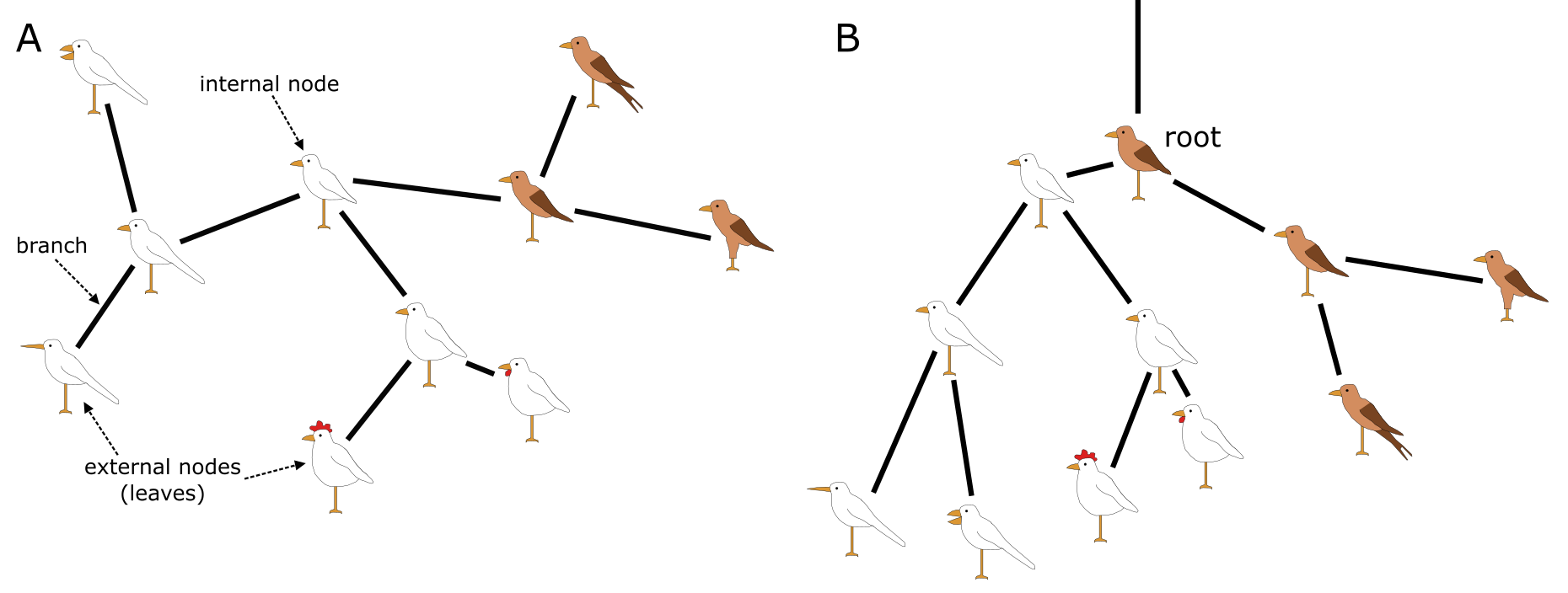
Figure 16:Rooting phylogenetic trees. (A) Unrooted tree depicting phylogenetic relationships among a set of white and brown bird species; external nodes represent the extant (living, observed) species, each with their morphological synapo- or autapomorphies, the internal nodes represent inferred (unobserved) ancestors. The tree is fully resolved, as each internal node is connected to three branches. Looking at the brown and white birds at adjacent internal nodes, it is not clear in what direction evolution proceeded and whether brown yielded white or rather the other way round. This becomes possible upon rooting the tree, usually based on comparison with an external reference species. (B) Rooted tree; external evidence (not shown) was apparently convincing in placing the root between the white and brown birds. Thus, a new, internally-placed, brown bird is inferred as the MRCA, making the brown birds paraphyletic with regards to the white birds, which are now monophyletic. Credits: CC BY-NC 4.0 Ridder et al. (2024)
Improper rooting affects clades and the overall structure of tree (as illustrated in Figure 17). The correct rooting of this tree is indicated, with human and chimpanzee as sisters, which is undisputed and based on external evidence for these species. Placing the root at the seven possible different positions in the unrooted tree of five terminals shows that only in three cases the (correct) human-chimp-gorilla monophyly is maintained (Figure 18). The other four topologies show extensive conflict, both with each other and with the correct topology. This indicates that care should be taken in selecting and assigning a suitable outgroup, which can be problematic in the case of isolated long phylogenetic branches (for instance, in protists or zooplankton lineages) or in the case of reconstructing a gene tree. In that case, one usually considers a copy of the gene of interest with sufficient similarity to be considered homologous, in a far-related evolutionary lineage (such as Amborella, for angiosperm plants) as a suitable outgroup for rooting that gene tree. Figure 19 shows an example of an unrooted tree with additive branch lengths.
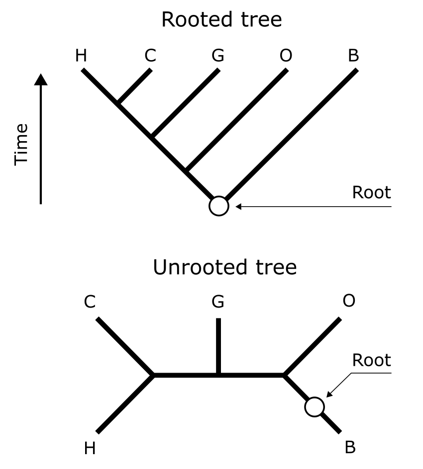
Figure 17:Rooting phylogenetic trees. With human (H), chimp (C ), gorilla (G), orang-utan (O) and gibbon (B) indicated, the rooted tree (top) represents the correct tree topology based on external evidence. The position of this root is indicated, both in the rooted and unrooted tree. Credits: CC BY-NC 4.0 Ridder et al. (2024).
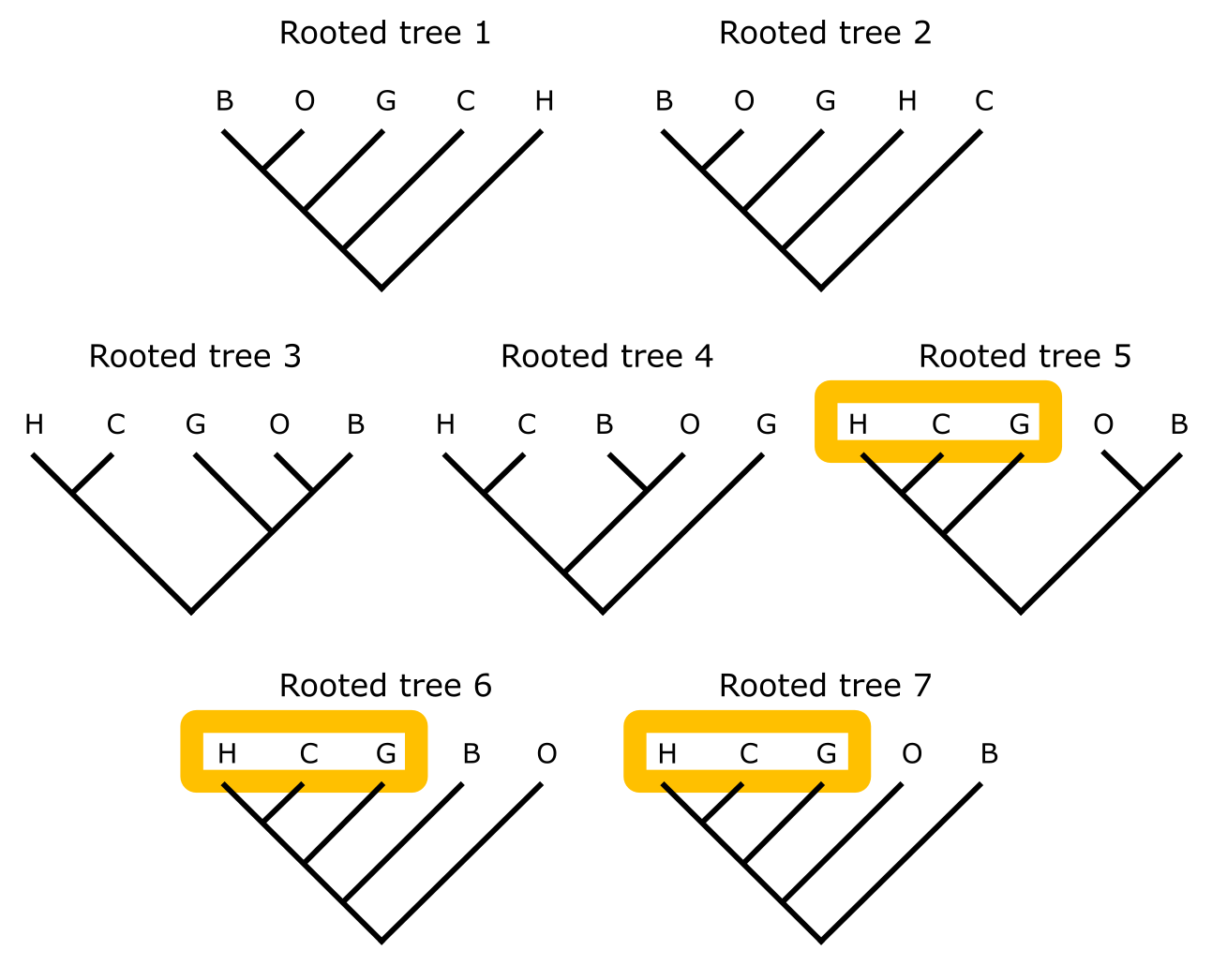
Figure 18:Rooting phylogenetic trees. The seven rooted trees that can be derived from the unrooted tree for five sequences in Figure 17. Each rooted tree 1-7 corresponds to placing the root on a different branch of the unrooted tree. Terminal labels as for Figure 17; the orange shape indicates monophyly of human, chimp, and gorilla, when present. Credits: CC BY-NC 4.0 Ridder et al. (2024).
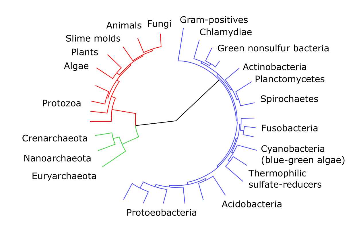
Figure 19:An example of an unrooted tree featuring groups of archea, bacteria and eukarya. color marks indicate groups that may be clans, depending on how the tree may become rooted. Credits: CC0 1.0 A1 (2009)
Newick tree notation
Phylogenetic trees are graphical structures (‘graphs’) that are the outcome of phylogenetic reconstruction of sometimes hundreds or thousands of sequences, and especially when using character-based tree search (see below Main approaches to tree building) there can be enormous amounts of ‘best trees’ that all will have to be taken into account, for instance by calculating a consensus tree (see Tree space and heuristic search methods).
In any case, handling large numbers of trees in phylogenetical and bioinformatic analytical pipelines requires the tree graphs to be in a format that can be easily read and produced, as a linear statement.
For this, the Newick notation is commonly used in which brackets describe the structure of the tree.
For instance, the rooted tree in Figure 17 above would look like ((((H,C)G)O)B) in Newick notation.
In case the tree has branch lengths, they can be indicated in this notation as well (see also the Newick tree Activity suggested on Brightspace).
Main approaches to tree building
Character based
Tree building is about finding clades and reconstructing phylogenetic relationships among a group of individuals. These individuals can represent genes, species or higher taxa, but they are never categories (or averages), as characters and states are observations on individuals. Considering one character (i.e., an MSA position, or column) at a time, Character-based methods, for instance maximum parsimony (MP), Maximum likelihood (ML) and Bayesian inference (BI), simultaneously compare all sequences in an MSA, in order to calculate a score for each character. The task is then to find the tree with the best overall score across all characters. This score, which is also known as an optimality criterion, is a measure of how well the data (the characters in your MSA) fit on to a particular tree under consideration. This is then repeated with another tree, and again another etc. -the better the fit, the better the tree.
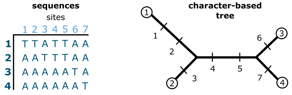
Figure 21:Character-based tree building. A DNA sequence data set (MSA) of 7 characters observed over 4 terminals (sequences) analyzed using a character-based approach (in this case: parsimony). Credits: CC BY-NC 4.0 Ridder et al. (2024).
In Figure 21 a DNA sequence MSA of 7 sites for 4 terminals is given, as well as a starting tree onto which each character is optimised. In this case the tree is ((1,2)(3,4)) but it could equally well have been any other tree for 4 terminals, the point being that it is a starting tree. Character 1 and 2 are autapomorphies, i.e., they occur only in one terminal (in this case terminal 1). This means that these two characters, like characters 3, 6 and 7, do not contribute to the structure of the (parsimony) tree but just elongate their terminal branches. Characters 4 and 5, however, are synapomorphies, they determine the internal structure of this tree. Across all characters, the total tree length is 7 steps, which would probably have been quite different using a tree with, for instance, ((1,4)(2,3)) as structure (or topology). There can also be multiple equally parsimonious trees as a result, which leads to the next issue: searching a tree space.
Tree space and heuristic search methods
The number of possible Bifurcating trees increases astronomically with increasing numbers of included taxa (terminals or sequences in your MSA) and cannot be calculated analytically (see Box 3.3). For instance, the total number of unrooted bifurcating trees for 10 and for 30 sequences is and respectively. In fact, it quickly becomes practically impossible to compare all possible trees and find the exact best one. To overcome this problem, random trees are generated that serve as starting points for tree search in remote and differently placed parts of the tree space. Different kinds of branch-swapping with local re-arrangements can be used to improve the tree score, and then the best-scoring trees (which can be many) are selected. Such tree search methods are called heuristic (rather than exact), yielding best possible estimates, though not necessarily guaranteed best solutions. Answers represent estimates, and whether or not the ‘best tree’ is actually found remains an open question.
These character-based tree building methods (as opposed to distance-based methods, below) are attractive in that trees are made directly from sequence characters, enabling detailed analysis of what characters contribute where in the tree, or reconstructing what ancestral characters (and hence sequences) would have looked like. This is a powerful feature of character-based tree building methods, which have become dominant in recent years.
Consensus trees
Following the character-based tree building approach does usually not result in just one best tree, but rather a set of trees that all score best under the optimality criterion applied. In such cases a Consensus tree will have to be calculated to efficiently communicate the outcome of the analysis. In Figure 23 three trees are shown, along with their so-called strict consensus and 50% majority-rule consensus trees which are explained below. Congruence among trees means that the same nodes (and hence clades) can be found in each tree. There may be differences, but these do not contradict the other tree topologies.
Trees 1, 2 and 3 are incongruent (i.e., they contain clades that contradict those in the other trees), therefore it is important to apply the right consensus approach in order to visualise the differences between the trees. Strict consensus demands that only identical tree topologies are visualised. As this is not the case (AB,C is present in Trees 1 and 3, but not in 2; ‘AB,C’ meaning there is a clade AB and C is its sister), this part of the strict consensus collapses into the trichotomy (A,B,C). Likewise, D and E are monophyletic only in Tree 3, therefore this part of the tree collapses in a ‘deep’ trichotomy (D,E, the rest). Strict consensus is therefore generally considered too strict, and losing information. For the 50% majority-rule consensus, which is most commonly used, the amount of (in)congruence among a set of trees is actually quantified, based on the occurrence of each node in the entire set of trees, and applying a majority-rule threshold. Thus, in Figure 23 clade AB occurs in Tree 1 and Tree 3 and its group frequency in the 50% majority-rule consensus tree is therefore ⅔ or 67% . Clade ABC is present in all trees and gets 100%. Clade ABCD is present in Tree 1 and Tree 2 and gets 67%. DE occurs only once and gets 33%, which is below the majority of 50% and therefore does not occur in the 50% majority-rule consensus tree.
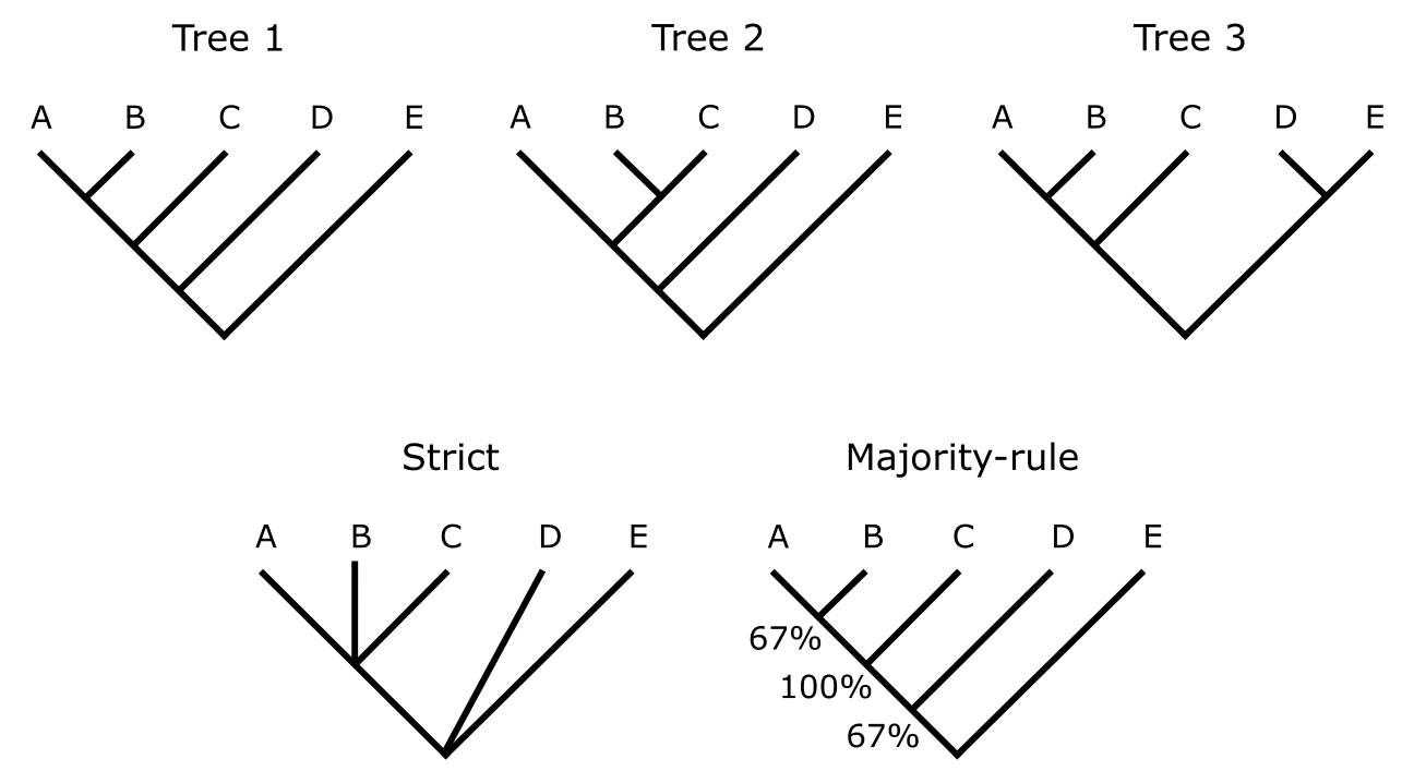
Figure 23:Consensus trees. Three primary trees are shown on top, their strict and 50% majority-rule consensus trees on the bottom. Credits: CC BY-NC 4.0 Ridder et al. (2024).
Parsimony analysis
The simplest method for character-based tree building is parsimony analysis in which, character-by-character, the fit (of each character) onto a candidate tree is counted (see Figure 24). Some characters may have changed only once but did so in multiple sequences (synapomorphies, whereas others may have changed several times independently (named homoplasies). Some characters may have changed only in one of the sequences (Autapomorphy). When all characters in the MSA have been evaluated, the overall score of the fit of the data with that candidate tree is calculated by adding up the changes across all characters (as in Figure 24). Then, another candidate tree is assumed and the process is carried out again. More and more trees are compared this way until either a single best or a group of equally most parsimonious reconstructions remains. Given the vastness of tree spaces for even moderate numbers of terminals (see Box 3.3) this process may take some time to complete. Usually only heuristic search methods (see Tree space and heuristic search methods) are applied in case of >15 terminals.
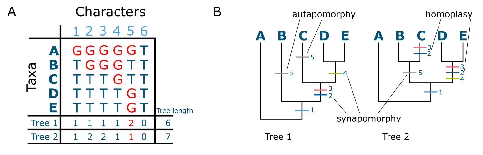
Figure 24:Parsimony analysis (same data and trees as in Figure 14). Character state changes (‘steps’) for all characters in the MSA shown left are indicated on the trees and exemplar syn- and autapomorphies are indicated. Note that character 6 is invariant and therefore does not contribute to any tree. Also note that each substitution occurring in the MSA results in one extra step on the tree. Credits: CC BY-NC 4.0 Ridder et al. (2024).
Each character change can be considered an ad hoc assumption, each of them associated with their type I error, i.e., the chance of having a false positive. This would be a character change (substitution) inferred on the tree where no change took place. The tree that minimizes the number of changes also minimizes the number of ad hoc assumptions, and hence the type I error.

Figure 25:William of Ockham, ‘father of parsimony’, from the 14th century. Credits: CC BY-SA 4.0 Mimi (2022).
This is the parsimony criterion, that was already described in the 14th century by the Franciscan friar William of Ockham (Figure 25) and has become known as ‘Occam’s razor’. In other words: when presented with competing hypotheses about the same prediction, one should select the solution with the fewest assumptions.
Is nature parsimonious? This is a commonly-heard question, probably inspired by the notion that Occam’s razor itself may be an assumption, but it is good to keep in mind that the parsimony criterion is only applied to choosing between hypotheses (i.e., trees) and does not assume anything about nature and evolution! Maximum parsimony methods are included in the software (MEGA11Tamura et al. (2021)) used in this chapter’s practical.
Two other important character-based methods for tree building exist: maximum likelihood (ML) analysis and Bayesian Inference (BI). Both differ from parsimony analysis in that they do not merely count differences (as in parsimony analysis) but are based on explicit models of character evolution and operate in a probability framework. ML will be discussed in section Maximum likelihood tree building below; BI is beyond the scope of this course and will therefore not be treated here.
Distance-based
The other main approach to tree building is clustering, which is distance-based, and is widely used in several applications, for instance in visualising BLAST searches as Neighbor Joining trees. In Distance-based methods, instead of comparing one character at a time across all sequences in the MSA, only pairwise comparisons of entire sequences are made (i.e., all characters are compared at once), for all possible sequence pairs in the MSA (Figure 26) typically yielding a triangular all-to-all distance matrix. Pairwise comparisons yield pairwise distances, which can be ultrametric or Euclidean (see Box 3.4). Keep in mind that the relation between Distance () and Similarity () is:
and that in different studies either or may be used for comparison. Which one is used can usually easily be inferred from the resulting pairwise distance matrix diagonals, where each sequence is compared with itself. There will be all 0’s in case of a Distance matrix and 1’s in case of a similarity matrix.
In (Figure 26), pairwise distances are calculated from the same MSA used in Figure 21 by counting the number of differences in each possible pair of sequences. This yields a triangular pairwise distance matrix, the values of which (the distances) are then used to build a distance tree, for instance using Neighbor Joining. The MSA is then not further used in the analysis. In this case the distance values perfectly fit the resulting distance tree.
Note that both trees in Figure 21 and Figure 26 have the same topology, but the parsimony tree contains more information: in addition to the branching pattern and branch lengths it also contains information on what character changed where on the tree.
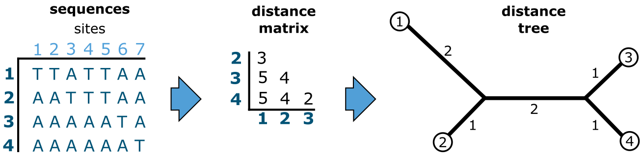
Figure 26:Distance-based tree building. The same data set (MSA) of 7 characters observed over 4 terminals (sequences) analyzed using a character-based approach in Figure 21, now using a distance-based approach. Credits: CC BY-NC 4.0 Ridder et al. (2024).
If the sequences would have accumulated substitutions in a clock-like manner (i.e., like radio-active decay) the resulting pairwise distances may even be ultrametric (see Box 3.4). This would mean that the distances in the triangular pairwise distance matrix are identical with the distances as measured over the resulting distance tree (Figure 26). However, such clean data is hardly ever found, and the distances measured over the tree may differ from the observed distances in the pairwise matrix. This is illustrated in Figure 27 in which two trees are depicted: an ultrametric tree (A) and an additive tree (B) containing unequal sister branch lengths (to a and b). In the additive distance matrix (matrix B), due to the difference in length towards a and b, the most similar sequences (i.e., b and c) may actually not be the most closely related (i.e., a and b).
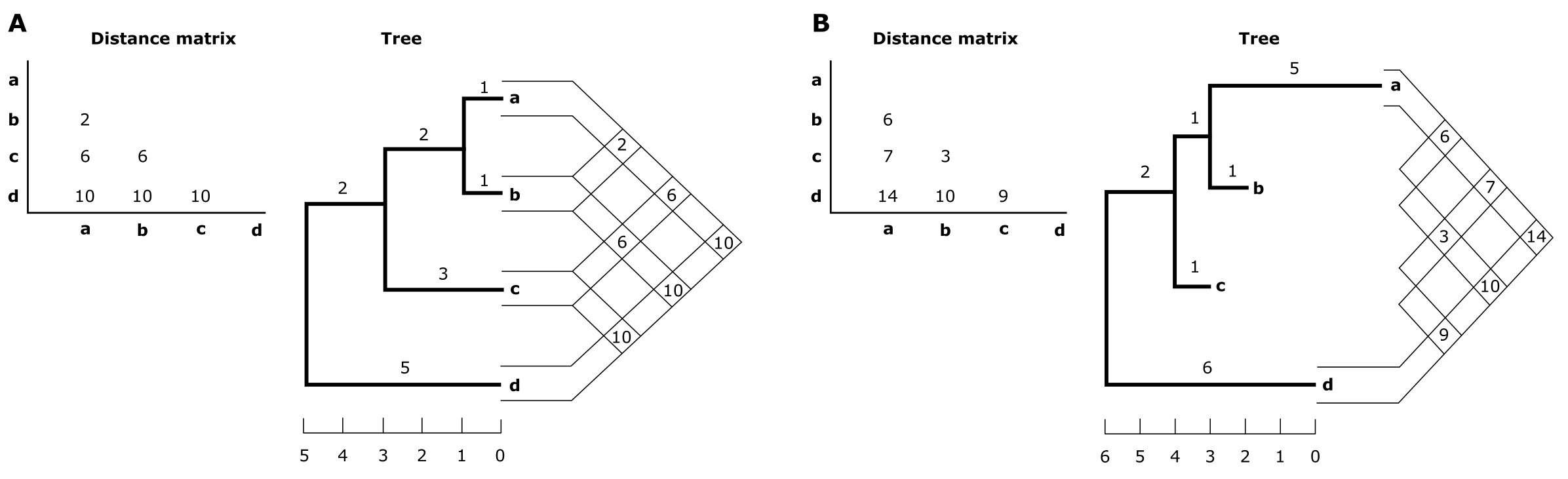
Figure 27:(A). Ultrametric distance matrix between four sequences a-d and the corresponding ultrametric tree. (B). Additive distance matrix between four sequences a-d and the corresponding additive tree. Values in the distance matrix correspond to the sum of the branch lengths along the path between the two sequences on the tree, therefore this data is metric. Note that in B, b and c are most similar, but not most closely related (a and b are). Credits: CC BY-NC 4.0 Ridder et al. (2024).
Once these pairwise distances have been calculated, the MSA is not further used and trees are built directly from the distances instead (Figure 26). Unlike for the character-based trees, in distance-based (clustering) trees it is not possible to assess what character contributed where on the tree, as all individual characters have been combined into one overall pairwise distance value. Moreover, invariant characters (MSA positions containing no variation) do contribute to the pairwise distance values. This is a main difference with the character-based approach where only variant characters contribute to the tree.
Clustering methods have the advantage that they are fast and do not require vast computational resources (there is no tree space nor NP-completeness as for the character-based trees, outlined above (see Box 3[w3box3_bifurcating])). Clustering methods assign individuals to clusters in such a way that individuals in one cluster are more similar to each other than to those from other clusters. There is no explicit score or optimality criterion, only the minimisation of overall distance across all sequences. Clustering usually produces one tree, no alternative ‘equally good’ trees are shown; this is due to the clustering algorithm which is designed to produce a single tree.
Neighbor Joining
Probably the most commonly used distance tree building method is Neighbor Joining (NJ), which is fast and effective, especially for large MSAs (with hundreds of sequences). NJ tree building starts with a fully unresolved tree, containing all sequences in the MSA, and calculates a total tree length (or overall starting distance) by summing all pairwise distances. Subsequently, a pair of sequences is chosen and combined to start a small cluster (‘neighbors’) and the total tree length is updated, now replacing the two original terminals by the joined neighbors. This step is repeated until all sequences and pairs are joined, whilst minimizing the overall distance (tree length) between them (Figure 30).
Neighbor Joining produces unrooted trees and therefore, if needed, outgroup rooting should be applied in order to root the tree. There is no molecular clock assumption, which allows differences in branch lengths between neighbors (sisters) to be reconstructed. NJ is implemented in MEGA11Tamura et al. (2021)) and used in the practical.
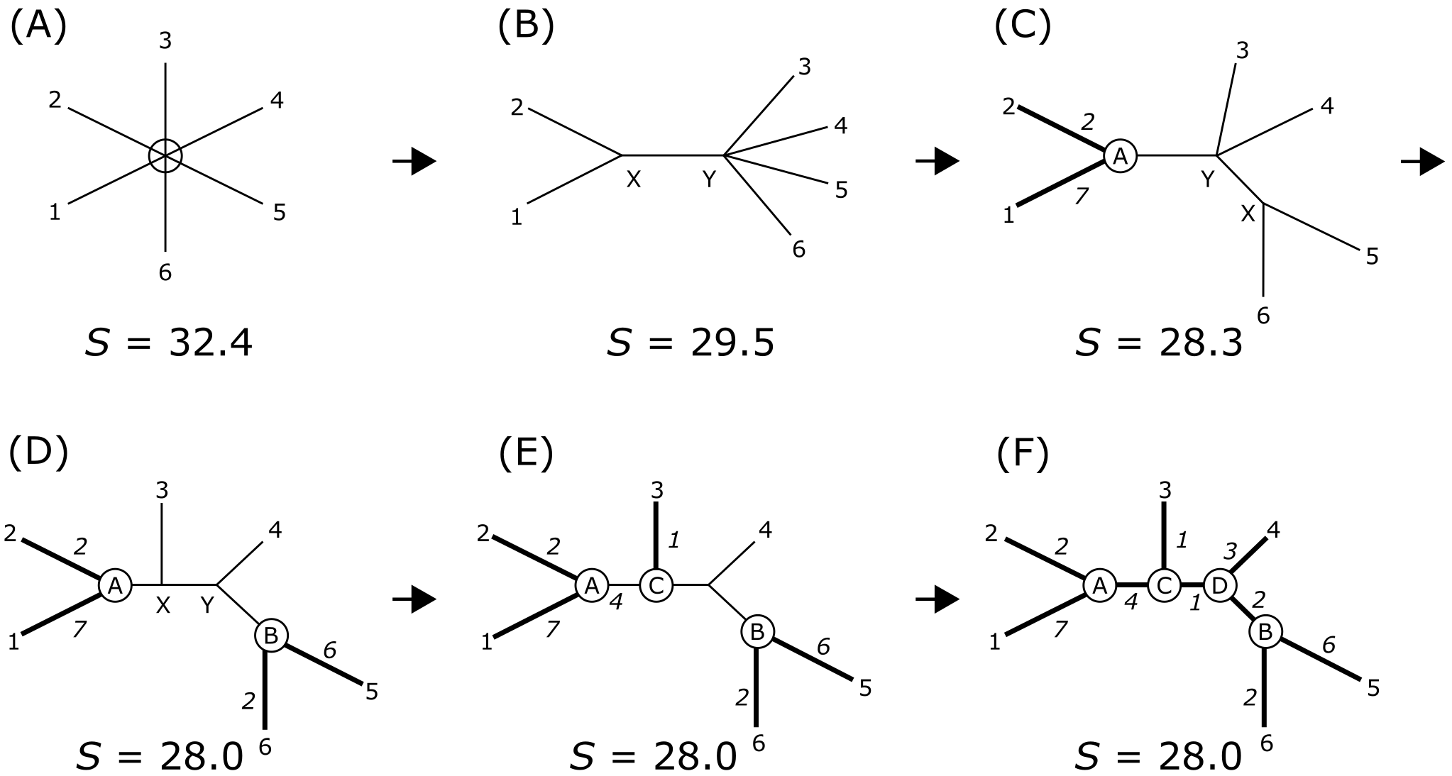
Figure 30:Neighbor Joining. An illustration of the computational process. Tree length S is the sum of all branch lengths, and is minimized (F) by iteratively joining neighbors, starting from the star tree (A). Credits: CC BY-NC 4.0 Ridder et al. (2024).
NJ is highly popular as it can generate trees with hundreds of terminals in a very short time. This makes it a great tool for quickly assessing the (phylogenetic) structure in a data set (MSA) without having to explore wide tree spaces (as in the character-based approach). It is good to keep in mind that NJ is a clustering method, i.e., it groups sequences on the basis of overall similarity, not on shared ancestry or Synapomorphy. Therefore, for phylogenetic studies, character-based analysis is preferred, and NJ analysis can be used in addition (Figure 31), to check for possible incongruencies between the two. If these are found, it could mean that the data (the synapomorphies accumulated in the MSA) are not metric for that part of the tree, which could warrant additional analysis methods (such as phylogenetic network reconstruction) which is beyond the scope of this course.
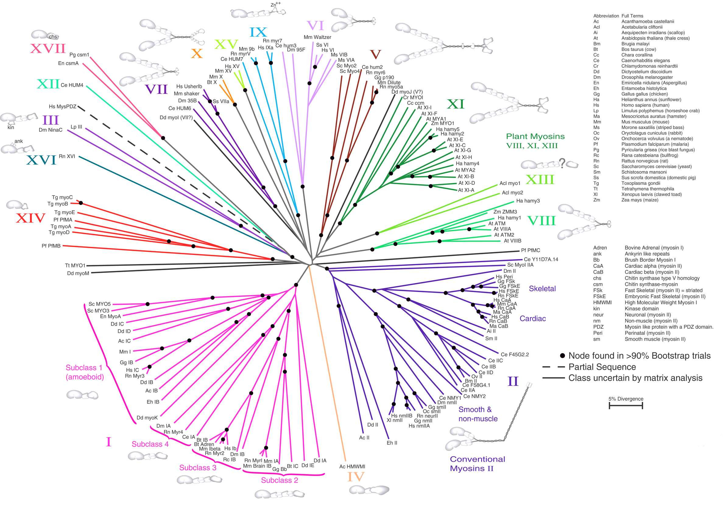
Figure 31:Neighbor Joining. An unrooted NJ tree based on Myosin amino acid sequences. The scale bar indicates 5% sequence divergence. Credits: CC BY 1.0 Hodge & Cope (2000).
Estimating sequence divergence
In a phylogeny, when there is a combination of long terminal branches combined with short internal ones, phylogenetic reconstruction is usually problematic when using nucleotides and parsimony analysis. The reason for this is that, when using a DNA MSA, on long branches (i.e., with highly-divergent sequences) the chance of any of the 4 nucleotides occurring in both branches at random, is actually quite high and can result in false synapomorphies. After some of these have accumulated, wrong clades can be the result. This so-called long branch attraction (LBA) artefact is fairly common, whenever isolated old lineages (such as Amborella or Nymphaea in the angiosperms) are involved but can also occur in gene trees. LBA has been shown to be mitigated to some extent by modelling branch lengths, rather than merely counting differences as branch length, as in parsimony where each substitution occurring in the MSA results in one extra step of treelength. For the accurate estimation of branch lengths in a phylogenetic tree however we need accurate sequence divergence estimation.
Evolutionary divergence (or distance) between homologous sequences is reflected in substitutions between them since splitting-off from their MRCA. Intuitively, when comparing two sequences, one would just take the proportion of differing sites as sequence divergence, for instance, for a sequence of 1000 positions, having 10 differences would yield 0.01 or 1% difference. However, this so-called p-difference does not necessarily consider all substitutions that historically occurred during divergence of the two sequences, which may include reversals to the original state. Estimating ‘true’ sequence divergence means that we need to find substitutions that did happen but are not visible in your MSA. Variable sites can actually keep on changing during evolution, causing multiple substitutions to occur at the same position, which can lead to saturation of change. In this way several substitutions may go unnoticed, and a mere p-difference will underestimate actual sequence divergence.
Substitution models
Substitution models, all based on the Jukes-Cantor (JC) formula given below, correct divergence estimates for unobserved events. The JC formula is based on calculation of the chance of having a substitution for a particular site plus the chance of it not changing into any of the three other nucleotides for that site. In the formula, stands for the observed proportion of differences (i.e., the p-difference), and for the corrected divergence measure. When all sites differ (i.e., ), reaches 0.75 in the limit, i.e., the corrected cannot exceed 75%.
Figure 32 shows how the JC formula is applied in a model of substitution, the JC model. There is a matrix defining the six possible substitution types among the 4 nucleotide bases, i.e., T↔C, A↔G, A↔T, T↔G, C↔G, and C↔A. In this case the relative rates for all six substitution types are assumed to be equal and denoted by one shared parameter, named ‘a’. Another assumption in this model is that the base composition across the MSA is equal, assuming a 25% probability of finding of each base at each position in each sequence. The JC model is considered a fairly simple, one parameter, model.
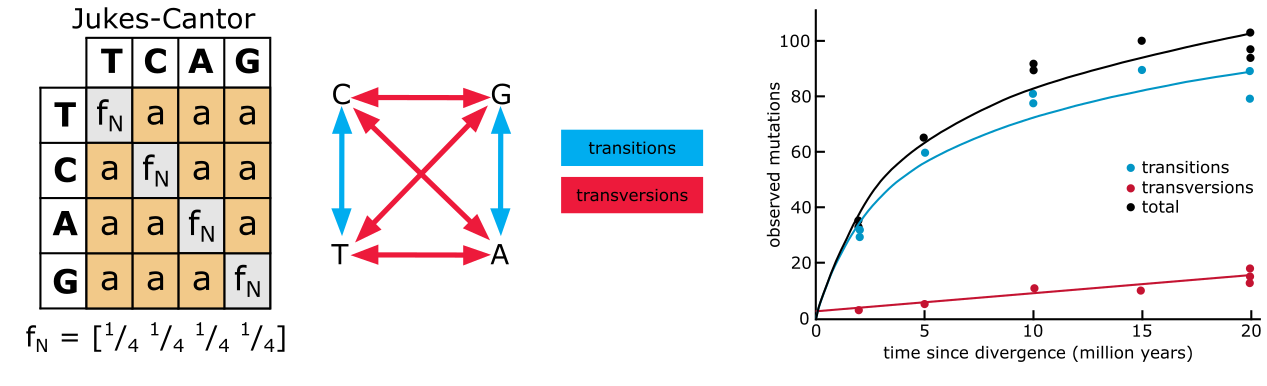
Figure 32:The Jukes Cantor model (left), transitions (blue) and transversions (red) and how they accumulate differently during evolutionary time (right). Credits: CC BY-NC 4.0 Ridder et al. (2024).
The first two substitution types listed above are Transitions_ (substitutions among the pyrimidines T and C, and among the purines A and G), whereas the other four occur between purines and pyrimidines and are referred to as Transversions_. The rate of transitions (ti) has a different dynamic, and hence build-up of substitutions, compared with the rate of transversions (tv) (see Figure 32). In the Kimura 2-parameter (K2P) model (Figure 33) this is accounted for by adding an extra parameter b. Parameter a now estimates ti () and parameter estimates tv (); in the Kimura 2 Parameter formula, and are the proportions of ti and tv, respectively:
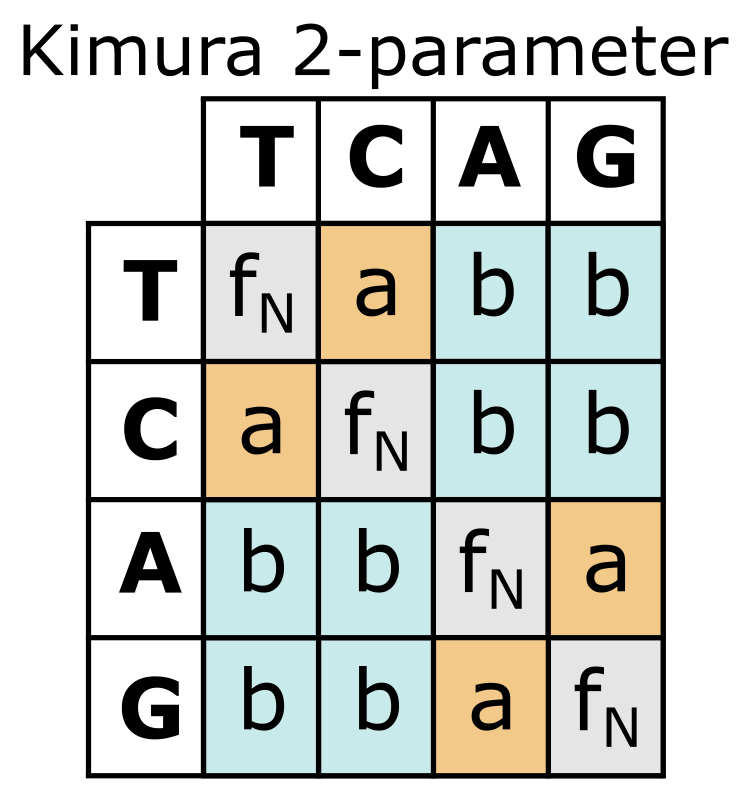
Figure 33:The Kimura 2-parameter substitution model with transitions indicated in orange (parameter a) and transversions in blue (parameter b). Note that base frequencies fN are considered equal in this model. Credits: CC BY-NC 4.0 Ridder et al. (2024).
Besides the JC and K2P models, other models exist that take into account different aspects of DNA sequence evolution, such as differences between all six substitution types (general time reversible or GTR), sequence base composition or nucleotide frequencies (Felsenstein81 or F81). Another aspect is the distribution of rates of change in sites throughout the MSA: how many fast, and how many slow-evolving sites are there and how are they distributed. This is achieved by comparison with a gamma Γ distribution (not shown). The most complex models, with many parameters, will consist of combinations of all these aspects of DNA sequence evolution. There are up to 220 different models to choose from. It is good to realise that these models are reversible and therefore allow the reconstruction of unrooted trees only. Once these are determined they can be rooted using outgroup rooting.
For amino acid sequence comparisons, instead of estimating parameter values from the data, amino acid substitution models are based on (pre-defined) substitution cost matrices (see chapter 2) that are based on observations of amino acid substitutions found in over 30,000 protein sequences (e.g., the JTT, Blosum, Dayhoff, LG and WAG matrices).
Maximum likelihood tree building
For character-based approaches these substitution models, as they are based on probabilities, allow us to calculate the likelihood of our data supporting a particular tree and model. This likelihood is a score describing how well data, tree and model fit together:
Or described in words: the likelihood is the probability of obtaining the data given hypothesis , which includes the substitution model and tree selected. We could therefore also say:
Obviously, it is important to select the best fitting model for the data set (MSA). Model selection proceeds by calculating the likelihood for your MSA using a range of different models and the same tree; the best resulting likelihood scores imply the best-fitting model.
Subsequently, a candidate tree is considered and the likelihood LD of observing the data (the MSA) is calculated given that model and that particular tree. Then, another tree is considered whilst the same best-fitting model remains selected, and its parameter values are estimated again. The likelihood LD of observing the data (your MSA) is calculated again and this time the likelihood may actually be better. More trees are evaluated, and more model parameter values are considered, all the time keeping track of LD until no further increase LD can be obtained. This is usually achieved by using the heuristic tree search approaches as outlined in Tree space and heuristic search methods and depending on the tree space, determined by the number of sequences in the MSA. The end result is the maximum likelihood estimate (MLE): the combination of a tree and model parameter values that maximizes the likelihood of the data. This tree, which may not be the exact best MLE (it is after all heuristics), is then usually referred to as the ML tree.
Phylogenetic tree reconstruction based on MLE has become the dominant tree building approach over the past decade. It is an efficient method that can consider differences in substitution rates and patterns between the sequences in an MSA. This would mean that non-clocklike or biased (non-random) accumulation of substitutions would be modelled, and this would minimize possible artefacts in inferring the ML tree topology, for instance LBA (see above).
The MLE pipeline for phylogenetic reconstruction is implemented in the software package IQ-TREE Minh et al. (2020), which includes I) model testing, II) ML tree search, and III) bootstrapping for both nucleotide and amino acid sequences. IQ-TREE will be demonstrated and used in this chapter’s practical.
Finally, estimating evolutionary divergence using nucleotide substitution models can also be applied in a distance approach. There, the substation models are applied to calculate ‘corrected’ pairwise sequence distances, which are then used to produce a Neighbor Joining tree (see Figure 30).
Model-testing, ML tree search, Bootstrapping
After an ML tree with branch lengths has been obtained, there is still no information on how nodes in the ML tree may differ in terms of support by the data (MSA). Therefore a bootstrap analysis is carried out, repeating the MLE process a number of times, based on pseudo-replicate data sets drawn from the MSA (see Nodal support in phylogenetic trees: the bootstrap). After an ML tree is obtained for each pseudo-replicate data set, a 50% majority-rule consensus tree is calculated in order to see the group frequencies (the proportion of replicates in which each node is occurring). These frequencies are also referred to as Bootstrap values. The idea is that the more synapomorphies a node has, the higher its bootstrap value will be.
Unfortunately, there is no simple linear relationship between character support and bootstrap values. Generally, bootstrap values < 90% are considered poor support for that node, and values < 50% (or even < 60%) as ‘no support’. Bootstrap values of 62% are usually obtained for MSAs containing one synapomorphy, meaning that such nodes should probably be ignored but this depends on the experience and interpretation of the analyst. Figure 34 illustrates what happens to bootstrap consensus trees when poorly supported nodes are collapsed: the tree topology becomes less well resolved but what is left is strong. That is indeed the trade-off: visualizing lots of nice but poorly supported resolution versus only focusing on strong nodes. Usually, we want to see both.
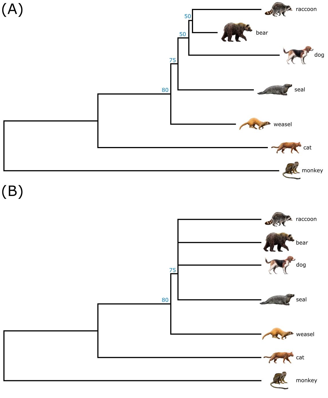
Figure 34:Bootstrap analysis. A) A maximum likelihood tree with bootstrap values indicated at nodes. Note that not all nodes show a bootstrap value, which is probably because values < 50% are ignored. B) The same analysis, but this time all nodes with bootstrap values < 50% are collapsed. Note the polytomy containing four lineages resulting from collapsing weak nodes; and note the change from additive tree to cladogram style in the collapsed tree. Credits: CC BY-NC 4.0 Ridder et al. (2024).
Recap tree building methods
To summarize, tree building methods can be classified according to the type of data used, characters (or ‘sites’) versus pairwise distance (clustering analysis). Using characters for tree building results in applying an optimality criterion in order to select among several (sometimes enormous numbers of) candidate trees. Clustering usually results in a single tree, the optimality criterion approach in several, in which case a consensus tree is calculated.
Another useful criterion to classify tree building methods is whether an explicit model of character evolution is applied, versus mere counting (parsimony) of changes. In this course we covered Maximum Likelihood and parsimony, and Neighbor Joining using corrected distances, i.e., applying the character model in pairwise sequence comparison. Bayesian Inference, in which probabilities for nodes are calculated, and different models are evaluated simultaneously, is beyond the scope of this course. (If you are interested, they are covered in BIS-40306 Comparative Biology & Systematics).
| Data → | Distances (pairwise) | Sites (characters) |
|---|---|---|
| Approach ↴ | ||
| Explicit model of character evolution | Neighbor Joining Neighbor Network | Maximum Likelihood Bayesian Inference |
| No model of character evolution | p-difference | Parsimony (‘counting’) |
| Optimality criterion | No, clustering | Yes, the tree length or likelihood |
Practical assignments
This guide contains questions and exercises to help you process the study materials of Chapter 3. You have two mornings to work your way through the exercises. In a single session you should aim to get about halfway through this guide, i.e., assignments I-IV. Note that assignment VI is optional.
These practical exercises offer you the best preparation for the project in week 6 and the tools and their use are also part of the exam material. Thus, make sure that you develop your practical skills now, in order to apply them during the project and to demonstrate your observation and interpretation skills during the exam.
Note, the answers will be published after the practical!
Glossary
- Additive tree
- A phylogenetic tree where branch lengths are proportional to the amount of change in the data.
- Autapomorphy
- Uniquely derived character state.
- Bayesian inference
- A character-based phylogenetic method that estimates posterior probabilities of trees given a model and data.
- Bifurcating
- A tree containing nodes that are all connected through three branches.
- Bootstrap
- A method for measuring node support in a phylogenetic tree.
- Bootstrap value
- Group frequency (percentage) with which a clade appears across bootstrap replicate trees.
- Branch length
- The length, either in steps (parsimony), distances (clustering) or substitutions per site (maximum likelihood) of a branch in an additive phylogenetic tree.
- Characters
- Observable features or traits of organisms. In molecular phylogenetics, each position in a sequence alignment (MSA) is treated as a character.
- Character-based methods
- Tree reconstruction methods that evaluate site patterns directly (e.g., parsimony, ML, Bayesian).
- Clade
- Monophyletic group, MRCA with all descendants.
- Cladogram
- A tree drawing showing topology only; branch lengths are not proportional to change.
- Consensus tree
- A summary tree of a set of equally good trees (e.g., strict consensus, 50% majority-rule).
- Distance-based methods
- Tree reconstruction based on pairwise sequence distances (e.g., Neighbor Joining).
- Gene duplication
- An event creating an extra copy of a gene in a lineage.
- Gene loss
- The disappearance of a gene copy from a lineage.
- Gene tree
- A phylogenetic tree reconstructed from gene (or protein) sequences, which may include paralogs.
- GTR
- General time reversible nucleotide substitution model.
- HTU
- Hypothetical taxonomic unit; an internal node representing an inferred ancestor.
- JC
- Jukes-Cantor nucleotide substitution model.
- K2P
- Kimura 2-parameter nucleotide substitution model.
- LBA
- Long-branch attraction.
- Maximum likelihood (ML)
- A character-based method selecting the tree and model parameters that maximize the probability of observing the data.
- MLE
- Maximum likelihood estimate.
- Monophyly
- For a group, all members being derived from one MRCA.
- MRCA
- Most recent common ancestor.
- Neighbor Joining (NJ)
- A distance-based tree building algorithm that iteratively joins neighbors to minimize total tree length.
- Newick
- A parenthetical text format for encoding tree topology (and optionally branch lengths).
- Nodal support
- The support—by the data—for a node in the phylogenetic tree (often measured by bootstrap values).
- OTU
- Operational taxonomic unit - used to classify groups of closely related individuals.
- Outgroup
- A reference taxon outside the group of interest used to root a tree.
- Paraphyly
- For a group, not all members being derived from one MRCA.
- p-difference
- Proportional difference, uncorrected.
- Phylogenetics
- The study of the evolutionary history and relationships among organisms or genes.
- Polytomies
- Parts of phylogenetic trees that are collapsed; nodes are connected through > three branches.
- Reconciled tree
- A gene tree interpreted alongside a species tree by adding duplications and losses to explain incongruences.
- Root
- Reference taxon or node used to polarize a tree.
- Rooting
- The act of assigning a root to a tree to infer direction of evolution.
- Sister group
- Two clades that share an exclusive MRCA with each other.
- Species tree
- A phylogenetic tree summarizing species relationships, potentially informed by multiple gene trees.
- States
- Specific conditions or manifestations of a character in a given individual or taxon. In molecular phylogenetics, each position in a nucleotide MSA (character) can have the state A, T, C or G.
- Synapomorphy
- Shared derived character state.
- Trait
- A distinct phenotypic characteristic of an organism, influenced by genetic and environmental factors.
- Transition
- A substitution among pyrimidines (C↔T) or among purines (A↔G).
- Transversion
- A pyrimidine ↔ purine substitution.
- Tree topology
- The branching structure of a phylogenetic tree, independent of branch lengths.
- Ultrametric inequality
- In any triplet, the two largest pairwise distances are equal.
- Ultrametric tree
- A rooted tree in which all paths from root to tips have equal length (interpretable in time units).
- Triangle inequality
- For any triangle with sides , , and , the sum of any two sides must be greater than or equal to the length of the remaining side:
- Huerta-Cepas, J., Marcet-Houben, M., & Gabaldón, T. (2014). A nested phylogenetic reconstruction approach provides scalable resolution in the eukaryotic Tree Of Life. PeerJ PrePrints, 2:e223v1. 10.7287/peerj.preprints.223v1
- Hadfield, J., Megill, C., Bell, S. M., Huddleston, J., Potter, B., Callender, C., Sagulenko, P., Bedford, T., & Neher, R. A. (2018). Nextstrain: real-time tracking of pathogen evolution. Bioinformatics, 34(23), 4121–4123. 10.1093/bioinformatics/bty407
- Ridder, D. de, Kupczok, A., Holmer, R., Bakker, F., Hooft, J. van der, Risse, J., Navarro, J., & Sardjoe, T. (2024). Self-created figure.
- DataBase Center for Life Science (DBCLS). (2023). Animal illustrations. https://togotv.dbcls.jp/pics.html
- DataBase Center for Life Science (DBCLS). (2021). Animal illustrations. https://togotv.dbcls.jp/pics.html
- Heled, J., & Drummond, A. J. (2009). Bayesian Inference of Species Trees from Multilocus Data. Molecular Biology and Evolution, 27(3), 570–580. 10.1093/molbev/msp274
- Tamura, K., Stecher, G., & Kumar, S. (2021). MEGA11: Molecular Evolutionary Genetics Analysis Version 11. Molecular Biology and Evolution, 38(7), 3022–3027. 10.1093/molbev/msab120
- A1. (2009). CollapsedtreeLabels-simplified. https://commons.wikimedia.org/wiki/File:CollapsedtreeLabels-simplified.svg
- Mimi, A. (2022). WILLIAM OF OCKHAM (1285 - 1347). English philosopher, also known as the “Invincible Doctor” (Doctor Invincibilis) and the “Venerable Initiator” (Venerabilis Inceptor). https://commons.wikimedia.org/wiki/File:GUILHERME_DE_OCCAM_(1285_-_1347)._Fil%C3%B3sofo_ingl%C3%AAs,_tamb%C3%A9m_conhecido_como_o_%22doutor_invenc%C3%ADvel%22_(Doctor_Invincibilis)_e_o_%22iniciador_vener%C3%A1vel%22_(Venerabilis_Inceptor),.jpg
- Hodge, T., & Cope, M. J. T. V. (2000). A myosin family tree. Journal of Cell Science, 113(19), 3353–3354. 10.1242/jcs.113.19.3353
- Minh, B. Q., Schmidt, H. A., Chernomor, O., Schrempf, D., Woodhams, M. D., von Haeseler, A., & Lanfear, R. (2020). IQ-TREE 2: New Models and Efficient Methods for Phylogenetic Inference in the Genomic Era. Molecular Biology and Evolution, 37(5), 1530–1534. 10.1093/molbev/msaa015
- Zvelebil, M., & Baum, J. O. (2007). Understanding Bioinformatics. Garland Science. 10.1201/9780203852507