2. Alignment, sequence search, and primer design
📘 This content is part of version: v1.0.0 (Major release)In this chapter you will learn about sequence alignment. During the practical you will learn how to make pairwise and multiple sequence alignments, perform sequence searches and motif analyses, design primers, and discuss the results.
Introduction
Comparing sequences is a key tool in the field of applied bioinformatics. By analyzing DNA and protein sequences, researchers can annotate genes in new genomes, build models of protein structures, and investigate gene expression. It is important to notice that nature tends to stick with what works, rather than reinventing the wheel for each species. Organisms evolve from ancestors and accumulate mutations. Here we deal with small-scale mutations, that affect a few characters: substitutions (see also Chapter 1) and small insertions and deletions (Figure 1). In chapter 5 we will also look at large-scale genome variations.
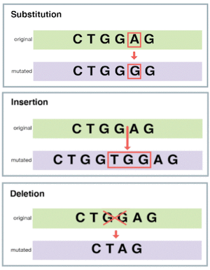
Figure 1:Different types of small-scale mutations.
Credits: https://
Via mutations, organisms can gradually develop new traits over time. These evolutionary relationships also mean that similar genes can be found in different organisms and the functional annotation can be transferred from one protein to another if both possess a certain degree of similarity. However, even though two proteins may look similar, they could have different functions. Generally, similarities arise because of shared ancestry (divergent evolution), nevertheless, similarities can also appear independently (convergent evolution). Before diving into the analysis of whether sequences are related, it is important to understand some key terms.
This chapter covers the basics of sequence comparisons. We will describe how two sequences can be compared with dot plots or with a pairwise sequence alignment. Then, the search of similar sequences in databases is described. Different approaches for comparing multiple sequences are covered: multiple sequence alignments to align them, motifs to find common sequences and profile hidden markov models to represent multiple sequences. This chapter concludes with a section on PCR primer design as an example on the use of sequence alignment algorithms in practice.
Dot plots
Dot plots are a simple way to visualize similar regions between two sequences. They are represented by a matrix, where one sequence is written vertically and the other horizontally. A dot is placed in a cell where the residues are identical. In the resulting plot, similar regions appear as diagonal stretches and insertions and deletions appear as discontinuities in the diagonal lines (Figure 2). A sequence can also be compared to itself, then the main diagonal will be filled with dots and additional repeats are on the off-diagonal (Figure 3).
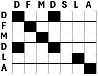
Figure 2:A small example of a dotplot.
Credits: CC BY-NC 4.0 Ridder et al. (2024).
Figure 3:An example of a dotplot to compare a sequence with itself. Credits: CC BY-NC 4.0 Ridder et al. (2024).
This simple way of marking identical residues comes with a lot of background noise. To detect interesting patterns, a filter is typically applied. For example, a minimum identity should be present across a certain window size, i.e., consecutive number of residues being considered. This feature is implemented in a webserver to visualize dotplots, dotlet Junier & Pagni (2000) (Figure 4).
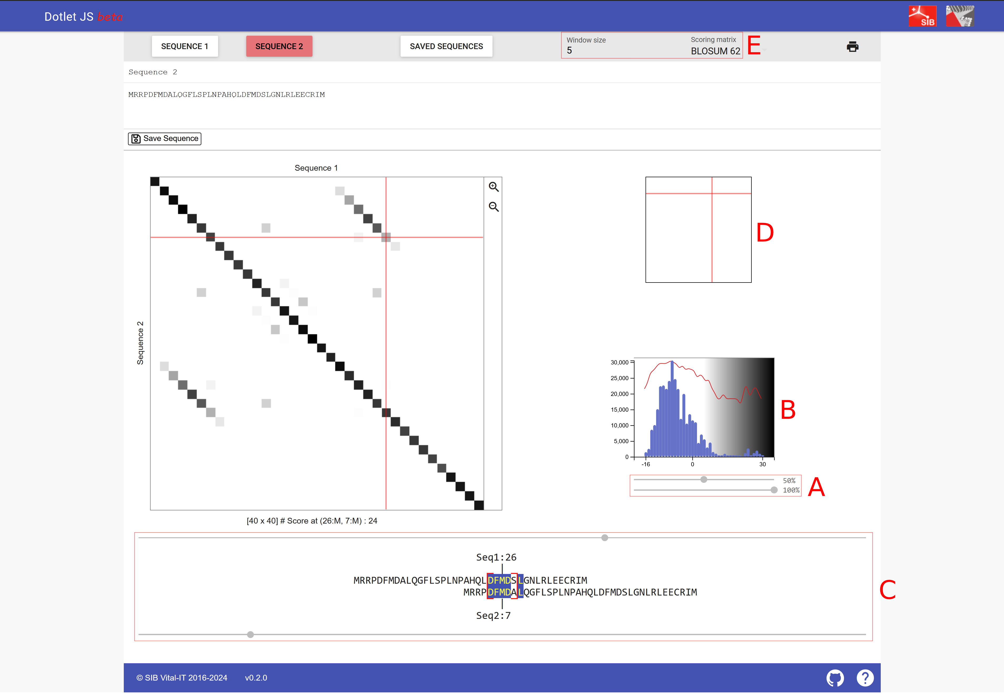
Figure 4:A screenshot of dotlet with the following protein sequence submitted as Sequence 1 and Sequence 2: MRRPDFMDALQGFLSPLNPAHQLDFMDSLGNLRLEECRIM.
- (A) The two sliders to change the appearance of the plot: The top slider can adjust the sensitivity, moving it to the right, fewer similar regions are shown; moving it to the left, also regions with lower similarity appear. The bottom slider adjusts the color scheme and is less relevant compared to the top slider.
- (B) The histogram indicates how many hits with a particular similarity are shown; thus the slider can be adjusted to the right tail of the histogram.
- (C) The two sliders that can adjust how the two sequences are positioned against each other.
- (D) Serves a similar function as the two sliders of C but allows for arrow key navigation of the dotplot.
- (E) Here you can select the window size of sequence comparison and the scoring matrix (window size is explained below and substitution matrices are also explained below).
- Credits: Junier & Pagni (2000).
Pairwise alignment
Dot plots provide a visual way to compare two sequences, but do not provide the similarity between two sequences. To calculate sequence similarity or sequence identity, we need to perform a pairwise sequence alignment. In an alignment, the two sequences will be placed above each other and gaps can be introduced to represent insertions or deletions of residues. We also say that the two sequences will be aligned. The resulting alignment contains matches, mismatches, and gaps (Figure 5)
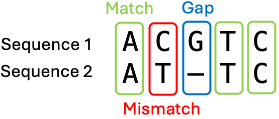
Figure 5:A small example of two aligned sequences. Credits: CC BY-NC 4.0 Ridder et al. (2024).
Alignments of DNA sequences
Every position in a sequence could potentially have an insertion or a deletion, so there are many possible locations and combinations for gaps and thus many potential alignments. The final alignment will be the one with the maximum total alignment score. This score is determined by so-called scoring parameters, which are chosen before the alignment calculation. An example of DNA sequence scoring parameters could be that matches score 1, mismatches -1, and a gap has a penalty of -1. The total score of an alignment is calculated by summing over all its columns (Figure 6). Then we can compare the scores of different alignments, where alignments with higher scores display a better alignment of the sequences. However, the choice of the scoring parameters has an impact which alignment will have the maximum score. To understand the impact of the parameters on the final alignment, fill in table Figure 7.
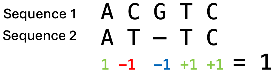
Figure 6:An example calculation of the alignment score, where matches score 1, mismatches -1 and there is a gap penalty of -1. This results in a total score of 1 for this alignment. Credits: CC BY-NC 4.0 Ridder et al. (2024).
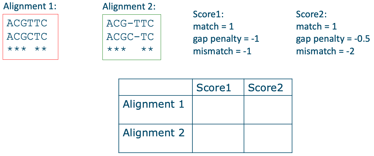
Figure 7:Assignment: Fill the table for the two alignments and the two sets of scoring parameters. Credits: CC BY-NC 4.0 Ridder et al. (2024).
Alignments of protein sequences
Substitution matrices
In Chapter 1, we learned that different amino acids have different chemical properties. When protein structure and function are conserved, it is more likely that an amino acid gets replaced by a chemically similar one than a very different one. When aligning protein sequences, we thus want to penalize the substitution of chemically dissimilar amino acids and reward the substitution of chemically similar ones. To this end, the score of matches and mismatches is generally determined by a substitution matrix, e.g., BLOSUM62 - BLOSUM (BLOck SUbstitution Matrix) (Figure 8). The substitution matrix and the gap parameters then determine the alignment score (Figure 9).
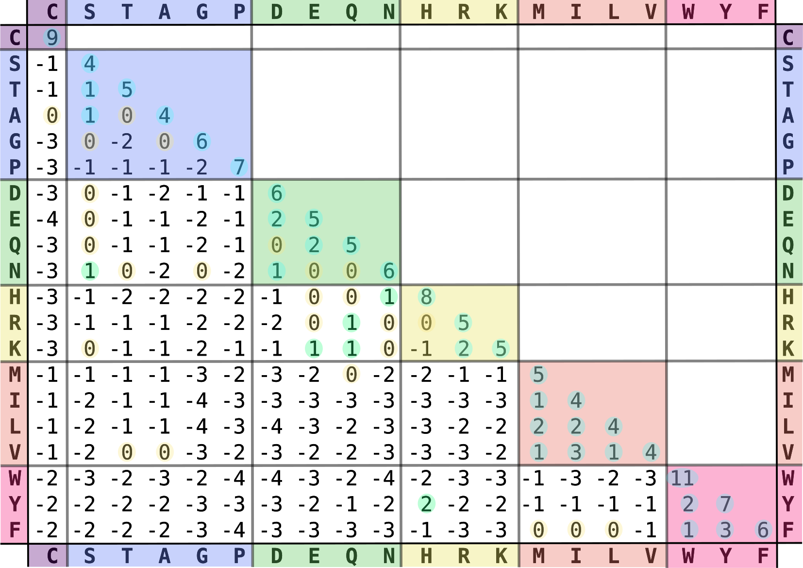
Figure 8:The BLOSUM62 amino acid substitution matrix. The matrix is ordered and positive values and zero values are highlighted. Credits: CC BY-SA 4.0 Ppgardne (2022).
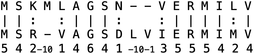
Figure 9:Example of a pairwise protein alignment. With the BLOSUM62 scoring matrix, a gap opening score of -10, and a gap extension score of -1, the resulting alignment score is 34. Credits: CC BY-NC 4.0 Ridder et al. (2024).
Note that we motivated the use of amino acid substitution matrices by the chemical properties of amino acids; however, these properties were not directly used when determining these matrices. Instead, the BLOSUM matrix is determined by aligning conserved regions from Swiss-Prot (Chapter 1) and clustering them based on identity. Then, the substitutions between the different pairs of amino acids within a cluster are counted, which is used to compute the BLOSUM scores. Thus, these scores reflect directly which amino acids are replaced more often with each other during evolution and we can observe that this frequency is strongly correlated with their chemical properties. There are different versions of BLOSUM; for example, BLOSUM62 was derived by clustering sequences with an identity of 62% and is appropriate for comparing protein sequences having around 62% identity. Other available matrices are for example BLOSUM45 (for more divergent sequences) and BLOSUM80 (for more similar sequences) (Figure 10).
Another group of matrices, that was derived even before BLOSUM, is PAM (Point Accepted Mutation). The entries in a PAM matrix denote the substitution probabilities of amino acids over a defined unit of evolutionary change. For example, PAM1 represents one substitution per 100 amino acid residues and is thus appropriate for very closely related sequences. A commonly used matrix is PAM250, which means that 250 mutations happened over 100 residues; that is, many residues have been affected by more than one mutation.
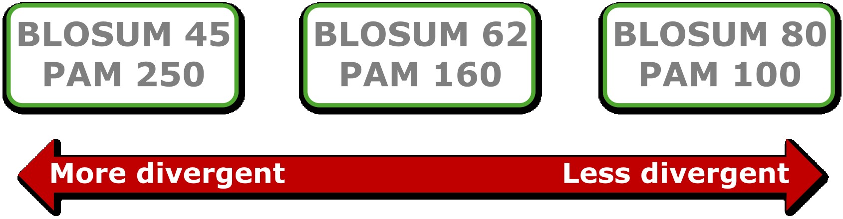
Figure 10:An overview of different available substitution matrices. Credits: CC BY-NC 4.0 Ridder et al. (2024).
Protein identity and similarity
For two protein sequences, we can distinguish two different measures of how much they are alike, identity and similarity, which are defined slightly differently. The protein identity is given by the number of identical amino acids divided by the alignment length. The protein similarity is given by the number of similar amino acids and the number of identical amino acids divided by the alignment length. In the pairwise alignment program needle, identical amino acids are marked by a vertical line ( | ), similar amino acids are marked by a colon (:) and defined by pairs that have a positive score (i.e., >0) in the chosen substitution matrix (Figure 11).
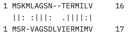
Figure 11:Example protein alignment. The percent identity is 10 / 18 = 55.6% and the percent similarity is 14 / 18 = 77.8%. The lengths of the individual sequences are shown on the right. Credits: CC BY-NC 4.0 Ridder et al. (2024).
Note that the pairwise alignment method does not directly try to maximize similarity or identity, but these calculated from the best alignment, which is a result of the chosen parameters. Especially for distantly related sequences, the parameters can have a big impact on the alignment and thus on the estimated identity and similarity. In Figure 12, you can find two alignments, where the same two protein kinases from rice have been aligned with different parameters. Depending on the parameters, the identity varies between 17.6% and 26.2%.
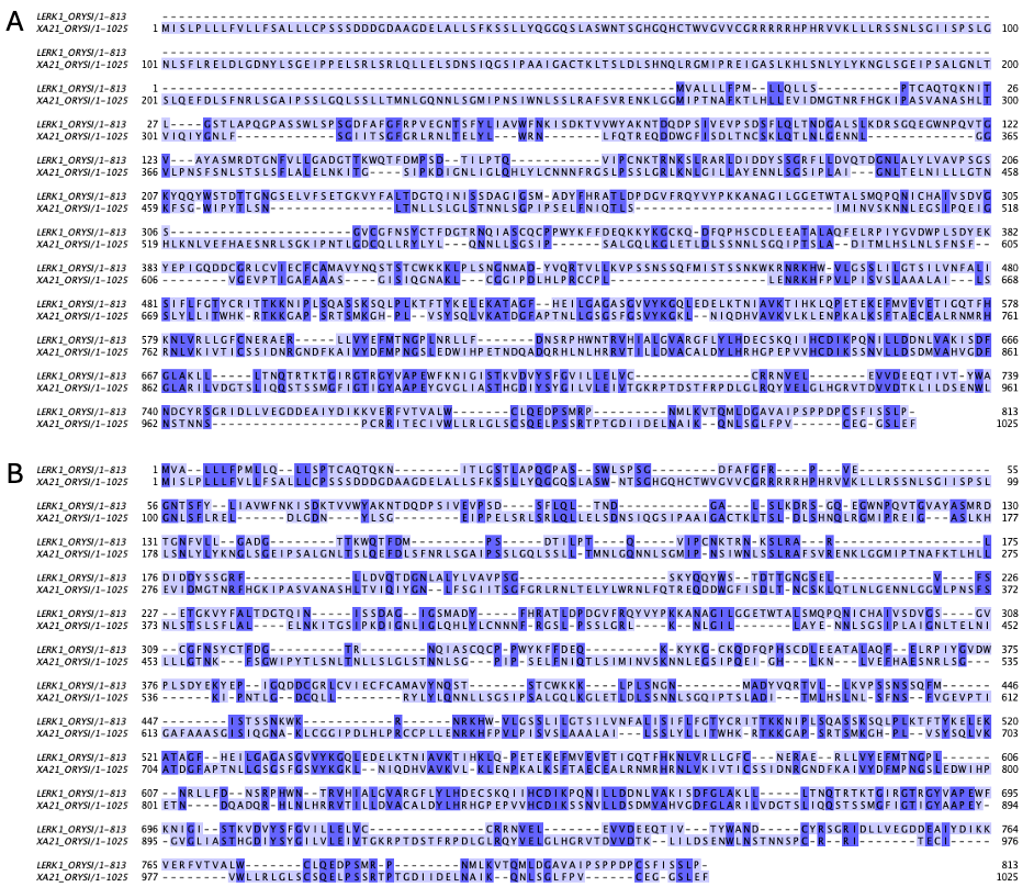
Figure 12:Alignments of the same two sequences (LERK1_ORYSI and XA21_ORYSI) with different parameters: A) BLOSUM62 matrix, gap open: -10, gap extend: -0.5. Identity = 210/1191 (17.6%), Similarity = 345/1191 (29.0%). B) BLOSUM62 matrix, gap open: -5, gap extend: -0.5. Identity = 305/1166 (26.2%), Similarity = 428/1166 (36.7%). Credits: CC BY-NC 4.0 Ridder et al. (2024) made using needle Madeira et al. (2022).
Up until now, we have only considered pairwise alignments, where both sequences are aligned completely; these are called global alignments.
Local alignments
We have seen in Chapter 1 that many proteins are composed of domains. Thus, some sequences might not be related over their full length, but only share similarity over parts of their sequences that correspond to domains. When comparing such proteins, it is more appropriate to perform a local alignment. Local alignment is also a good tool for identifying functional sites from which sequence patterns and motifs can be derived (Figure 13).
The aim of a local alignment is to find the best subsequences of both input sequences that result in the maximum alignment score given the alignment parameters. As for global alignment, efficient algorithms exist to solve this task. The Smith-Waterman algorithm can solve this task in a time that is quadratic in the length of the input sequences, just like the Needleman-Wunsch algorithm for global alignments.
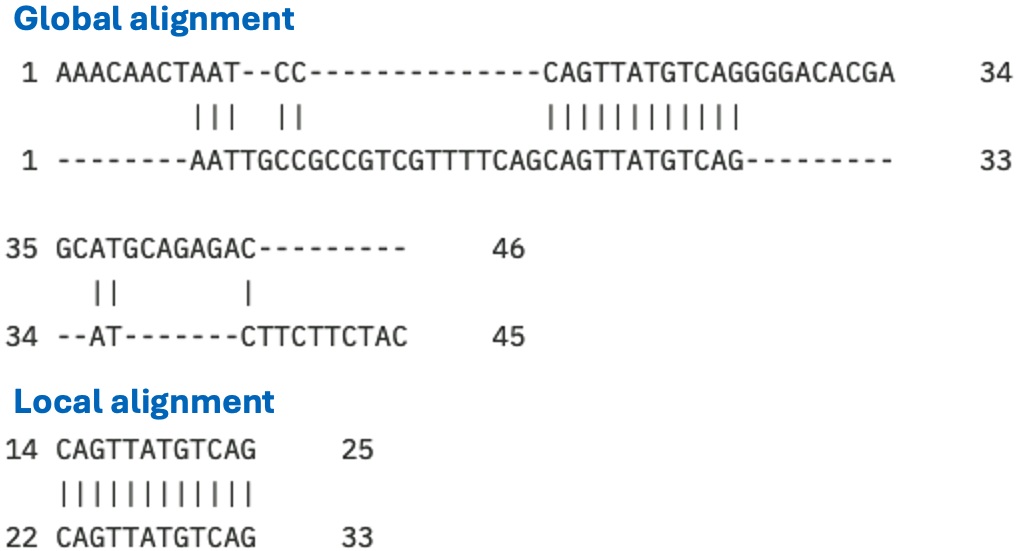
Figure 13:Alignments of the same two sequences, once using the global alignment program needle and once using the local alignment program water Madeira et al. (2022). The same alignment parameters were used: DNAfull matrix, gap open -10, gap extend -0.5. The global identity is 20/71 (28.2%) and the local identity is 12/12 (100.0%). Credits: CC BY-NC 4.0 Ridder et al. (2024).
Search in sequence databases
In Chapter 1, we learned about different sequence databases. We often want to search novel sequences in these databases, for example, to learn which other organisms have homologs. Two sequences that are highly similar might also share the same function. This relationship is used for the functional annotation of sequences, where the search in databases is an important step.
Database search vs. pairwise alignment
Pairwise alignments are also used when searching sequences in databases. In this task, we have a query sequence and we want to find similar sequences in a database; these similar sequences are called subjects or hits. Although the algorithms that were discussed in the previous section are relatively fast when two sequences are aligned, it would still take too long overall to perform pairwise sequence alignments of the query with all potential subjects from the database. We thus need even more efficient algorithms.
BLAST
Basic Local Alignment Search Tool (BLAST) is a heuristic method to find regions of local similarity between protein or nucleotide sequences. The program compares nucleotide or protein sequences to sequences in a database and calculates the statistical significance of the matches. Both the standalone and web version of BLAST are available from the National Center for Biotechnology Information (NCBI).
The algorithm
The starting point of BLAST is the set of words that two sequences have in common, where a word is a part of a sequence of a fixed length. For protein blast, the default word size is 5 and for nucleotide blast it is 11. To find these common words, first a lookup table of the query words is reconstructed (Figure 14A), where neighborhood words are listed as well. Neighborhood words are all the words that have a high alignment score with the query word (Figure 14B). Then, BLAST scans the database for word matches. For protein blast, two matches within 40 residues must be found for BLAST to consider it as an initial hit (Figure 14C). Note that for nucleotides, initial hits are found in a simpler way: only one exact match must be found, i.e., no neighborhood is considered.
After finding initial hits, BLAST extends these to local alignments (Figure 14D). As this extension happens, the alignment score increases or decreases. When the alignment score drops below a set level, extension stops. This prevents the alignment from stretching into areas where there is very little similarity between the query and hit sequences. If the obtained alignment receives a score above a certain threshold, it will be included in the final BLAST result. BLAST is thus a heuristic algorithm (Note 2.4), but its careful process provides a reasonable trade-off between run time and accuracy.
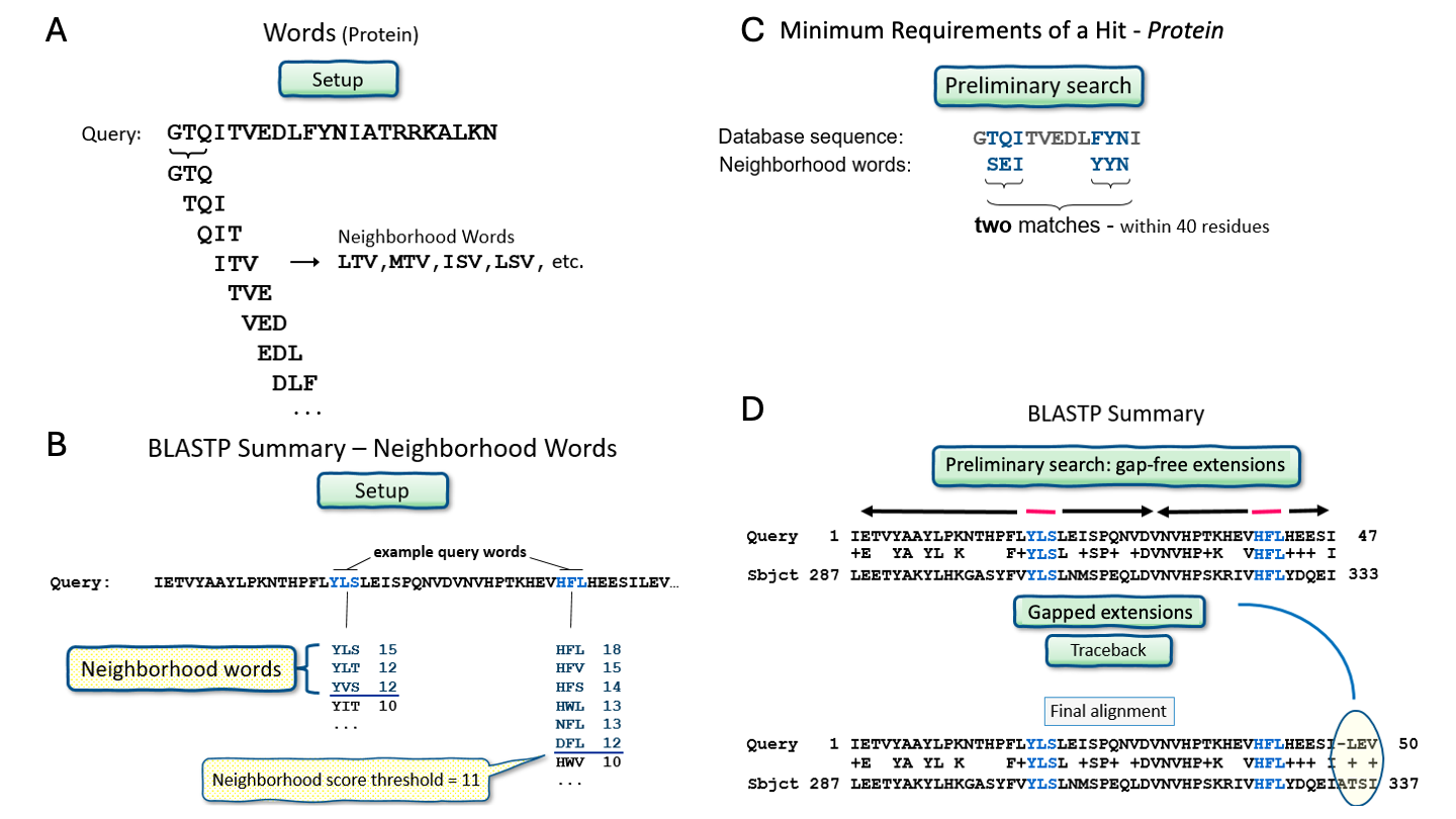
Figure 14:An overview of the BLAST algorithm. Credits: CC0 1.0 National Library of Medicine (NLM) (2022).
BLAST output
The BLAST output contains vast information on the found hits, their alignments, and taxonomy (Figure 15).
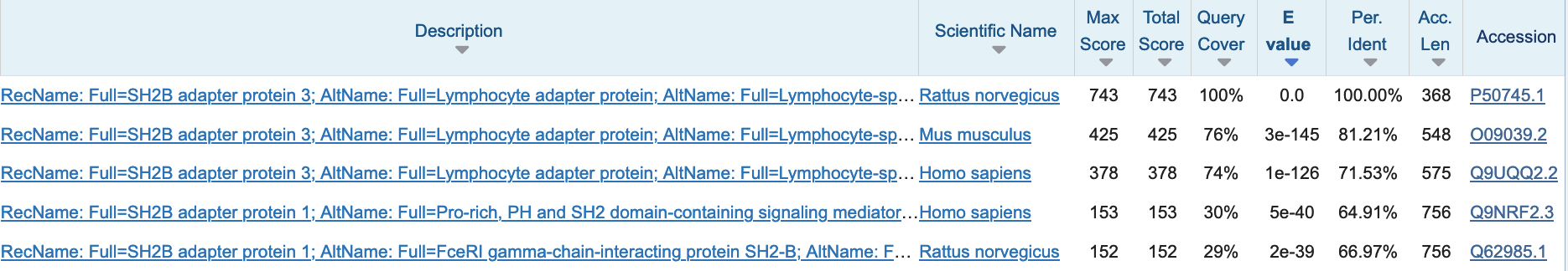
Figure 15:Top 5 blast hits when searching the rat protein P50745 in the Swiss-Prot 2024_02 release database. Credits: Camacho et al. (2009)
Note that you cannot infer homology by E-value alone; the coverage and percent identity need to be taken into account as well. For example, in Figure 15, all hits have very low E-values: the first hit is to the sequence itself; then there are hits with high identity and high coverage in mouse and human, these might be homologous sequences. The 4th and 5th hit are local, since the query cover is ~30%, these sequences might only share a homologous domain with the query protein.
BLAST types
Different types of BLAST exist to search nucleotides or proteins in the respective databases:
blastn searches a nucleotide sequence in a nucleotide database and blastp searches a protein sequence in a protein database.
In addition, the query and/or the database can also be translated in all six reading frames to allow additional kinds of comparisons (Figure 16).
Different BLAST types exist for these different kinds of comparisons, where these translations are done automatically (Figure 16).
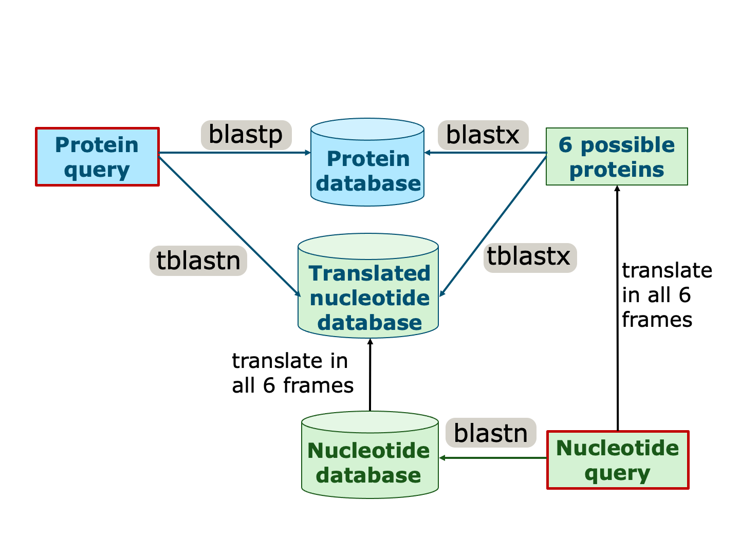
Figure 16:Different BLAST types to compare different data types. The input query is marked by a red box. Sequences/databases with a blue background originate from protein sequences, wheres sequences/databases with a green background originate from nucleotide sequences. Note that some of the latter are automatically translated into all possible proteins (indicated by blue font). Credits: CC BY-NC 4.0 Ridder et al. (2024).
PCR primer design
A special use case of sequence comparisons is designing primers for the polymerase chain reaction (PCR, see box 2.6). Many laborary techniques in biomedical applications rely on PCR for amplifying specific fragments of DNA. Examples include pathogen detection, analyzing genetic variation, targeted mutagenesis, de novo protein synthesis, and studying gene expression patterns. Which DNA fragments are amplified is determined largely by which PCR primers are used. To design primers that successfully amplify the DNA of interest, several computational steps are combined. This section highlights some of these bioinformatic considerations.
PCR primers typically have to meet several requirements to result in a successful PCR product: they have to be biochemically feasible (i.e. denature, anneal, and extend at the right temperature), they have to be specific (only amplify the region of interest), they should produce a product of a reasonable size (~500-1000 nucleotides, depending on the application), and they should be stable as single stranded DNA. The combination of these requirements typically allows primers of ~18-30 nucleotides long. To aid in the quick design of potentially successful primers, tools such as Primer-BLAST or Primer3+ automatically check most of the mentioned requirements. For example, Primer-BLAST lets a user upload a sequence of DNA that should be amplified, and can be configured to find primer products of a specific size. In addition, putative off-target amplification (to ensure specificity) is checked using BLAST on a database of choice, and several desired temperatures can be configured.
Comparisons of multiple sequences
Multiple sequence alignment
One straightforward observation from a sequence search is that one query sequence is often similar to multiple sequences (Figure 15). This can lead to research questions on evolution (where do these sequences come from?), function (why are some sequences more similar to each other than to others?), or structure (are all parts of these sequences equally similar/dissimilar?). Comparing all of these sequences with each other using a pairwise alignment strategy would quickly lead to a large number of comparisons and would be difficult to interpret. Instead, in cases where we want to compare 3 or more sequences with each other, we use a multiple sequence alignment (MSA).
The objective of performing multiple sequence alignment is to identify matching residues (DNA, RNA, or amino acids) across multiple sequences of potentially differing lengths. The resulting alignment can be thought of as a square matrix: rows represent the sequences that we started with, columns represent homologous residues across sequences, and the entries are either residues or gaps (Figure 18).
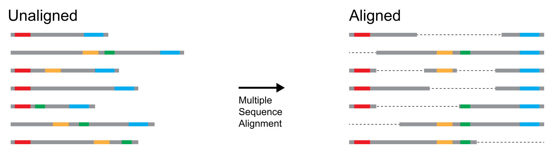
Figure 18:Conceptual diagram depicting multiple sequence alignment. Colored dots represent similar sequence elements, in the multiple sequence diagram on the right these elements align in vertical columns. Credits: CC BY-NC 4.0 Ridder et al. (2024).
In contrast to pairwise alignment, it is computationally not feasible to calculate the best multiple sequence alignment for a set of sequences and scoring parameters. Instead, various heuristic algorithms (Note 2.4) for creating multiple sequence alignments exist. Here we will go over two main concepts that are adopted by many tools: progressive alignment and iterative alignment.
Progressive alignment
Progressive alignment builds the alignment using a so-called guide tree (Box 2.2). The guide tree is a crude representation of similarity between all sequences to be aligned. Progressive alignment picks the two most similar sequences using the guide tree and initializes the multiple sequence alignment by aligning these two sequences with a global alignment strategy. Subsequently, the guide tree is used to determine the order in which sequences are added to the alignment. One way of thinking about this is that progressive alignment creates increasingly large ‘blocks’ of sequences, where a block is always treated as a unit (e.g., introducing a gap will happen for all sequences in the block). By going through the guide tree, this alignment strategy progresses to the final result, hence the name progressive alignment.
Iterative refinement
One potential downside of the progressive alignment strategy is that some of the intermediate blocks may represent sub-optimal alignments. For example, when a gap is introduced during an early stage of the progressive approach, it is never removed from the alignment. Identifying and potentially improving such cases is often referred to as iterative refinement and typically happens on a multiple sequence alignment that was created with a progressive strategy.
Iterative refinement takes as input a multiple sequence alignment, a scoring function for the multiple sequence alignment, and a function to rearrange the multiple sequence alignment. It produces a refined multiple sequence alignment by rearranging the multiple sequence alignment and only keeping the new multiple sequence alignment if the score has increased. This process is typically repeated until the score no longer increases (or for a fixed number of iterations).
Since iterative refinement methods typically start with a progressive alignment and improve its score, programs that implement an iterative refinement strategy (e.g., the FFT-NS-i method in mafft) typically perform better, but also need more time, than programs that are based on progressive alignment (e.g., the FFT-NS-2 method in mafft and the Clustal program) Katoh & Standley (2014).
Motifs
Having established how to obtain a multiple sequence alignment, we now focus on several interpretations. One possible interpretation is the identification of (and search for) commonly occurring sequence patterns. A frequently used term for a commonly occurring sequence pattern is motif, which we will use from now on. Motifs can be found by summarizing the columns of the multiple sequence alignment, in an attempt to describe commonly occurring residues across all sequences.
The simplest representation of a motif is the consensus sequence (Figure 19B), where every column of the multiple sequence alignment is represented by the most frequently occurring residue (i.e., the majority consensus). The downside of a consensus sequence is that it does not represent any of the variation present in the motif.
An extension of the consensus sequence that can represent some variation in a motif is the pattern string (Figure 19C).
In pattern strings, unambigous positions are represented by single letters and there is a special syntax for representing variation:
Positions in the MSA with more than one character are represented by multiple characters in between square brackets.
A pattern string containing, for example, the pattern [AG] indicates that one position in the motif can be either A or G.
As such, pattern strings take inspiration from regular expressions.
Various types of pattern strings exist; for example, PROSITE REF strings used in the Prosite database contain the syntax for representing positions in a motif where the residue is irrelevant (marked by an *).
Pattern strings are capable of representing some variation in the motif, but they cannot express how likely the occurrence of specific variants is (in the example of [AG], both A and G are equally likely to occur).
To express the likelihood of a specific residue occurring at a specific position, a Position Specific Scoring Matrix (PSSM) can be used (Figure 19D).
Every row represents one of the possible characters in the MSA and every column represents a column in the MSA, where numbers indicate the probability of observing a specific character at a specific position.
Hence, every column sums to one.
For example: a DNA PSSM would have four rows, representing the nucleotides A, C, G, or T.
The entries represent probabilities of observing a specific residue at a specific position.
As a consequence, all columns in a PSSM must sum to one.
Since a PSSM contains probabilities, it is relatively straightforward to calculate how well an unknown sequence matches an existing PSSM: assuming independence between positions, one simply multiplies the observation probabilities of the characters in the novel sequence.
Finally, sequence logos are a graphical representation of an alignment (Figure 19E). Every position in the sequence logo represents a position in the MSA. The total height of the logo at a position indicates the information that this column contains, i.e., an unambiguous position has a high information content, whereas a position with equal frequencies of characters has a low information content. Additionally, the characters are scaled proportional to their probability of being observed at their respective positions.
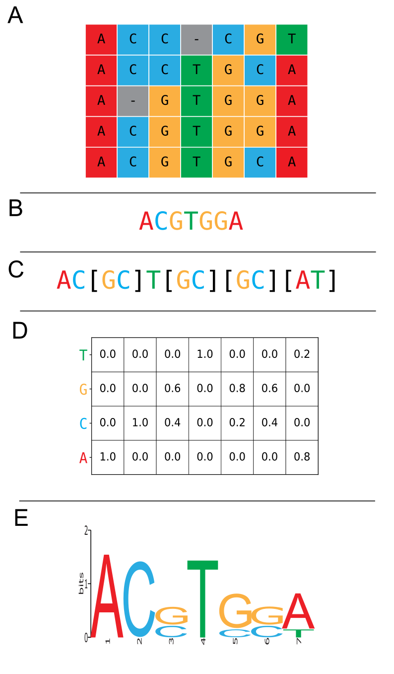
Figure 19:Conceptual diagram depicting various representations of a conserved motif. A: Multiple sequence alignment (MSA) of 5 sequences and 7 positions. B: Consensus sequence. C: Pattern string. D: Position Specific Scoring Matrix (PSSM). E: Sequence logo. Credits: CC BY-NC 4.0 Ridder et al. (2024).
Profile hidden Markov models (pHMMs)
The previous sections on multiple sequence alignments and motifs explained some basics of how collections of similar sequences can be summarized and used. In this section, we highlight a powerful approach for using the information in MSAs to perform sequence search and comparison: profile hidden Markov models (pHMMs). Some of the fundamentals of general hidden Markov models have been covered in Chapter 1; here we introduce how a few simple adaptations to the general concept of HMMs unlocks a powerful sequence search approach.
We can think of a profile hidden Markov model as an extension of a position specific scoring matrix. Like a PSSM, a pHMM contains probabilities of observing certain characters at certain positions in an MSA. However, in contrast to PSSMs, HMMS can also represent insertions and deletions, that is, an insertion at a particular position might be more likely than an insertion at another position. To this end, hidden Markov models contain the hidden states match/insertion/deletion and transition probabilities between the hidden states. In addition, emission probabilities represent the unique probabilities for the different characters for the match states and for the insert states. A graphical representation of a simple profile HMM can be seen in Figure 20. Just like for PSSMs, a probabilistic score can be calculated for a novel sequence matching an existing HMM. Efficient algorithms for working with pHMMs exist and have been implemented in for example the HMMer suite.
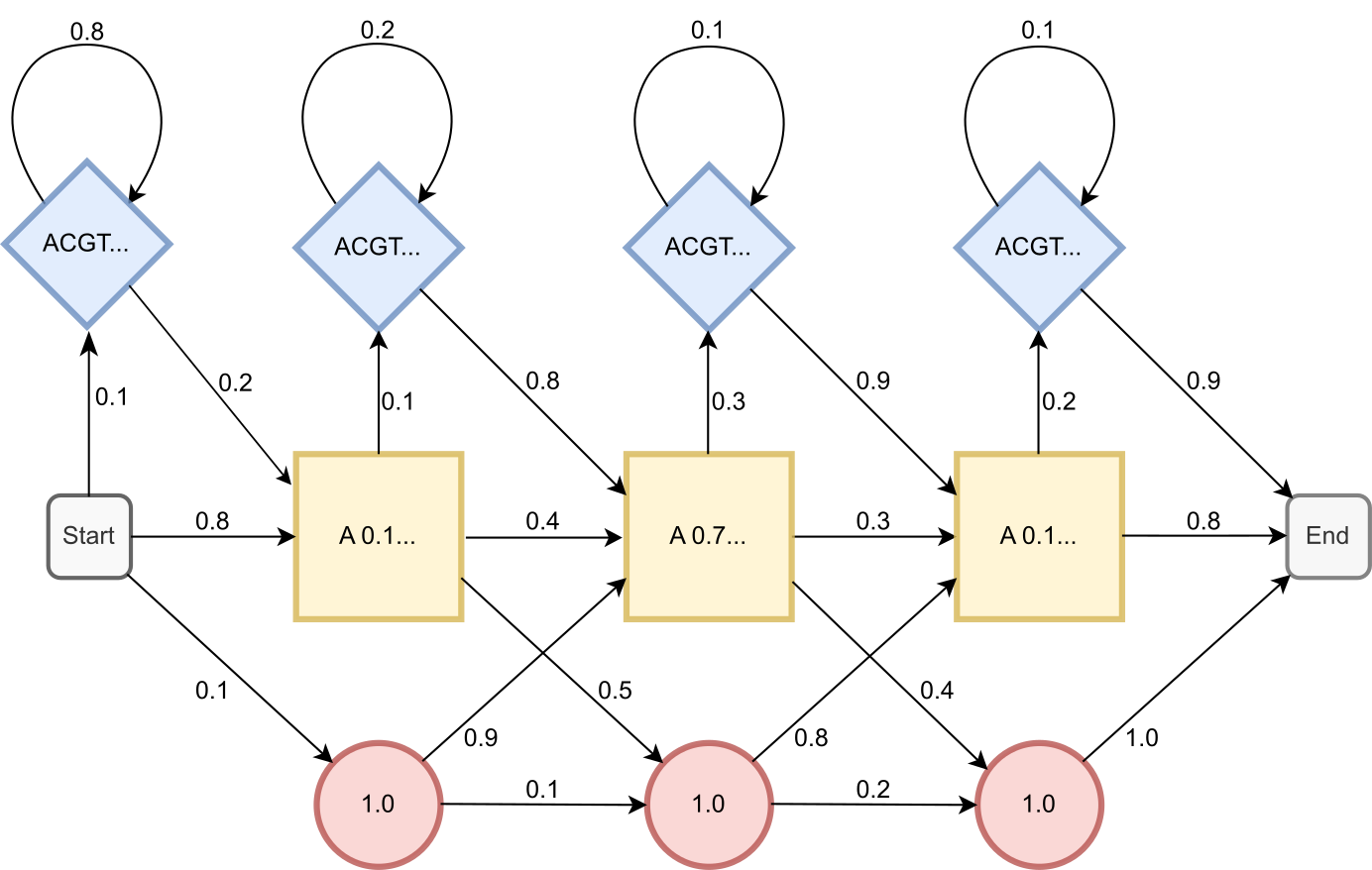
Figure 20:Schematic representation of a simple DNA profile HMM containing all model probabilities. The model consists of three types of hidden states: match (yellow square), deletion (red circle), and insertion (blue diamond). Emission probabilities are indicated inside the hidden states, transition probabilities between hidden states are indicated next to arrows. Credits: CC BY-NC 4.0 Ridder et al. (2024).
Practical assignments
This practical contains questions and exercises to help you process the study materials of chapter 2. There are two supervised practical sessions, one on Wednesday and one on Thursday. On the first practical day you should aim to get about halfway through this guide. Thus, you should aim to be close to finishing Exercise 4 on the first day. Use the time indication to make sure that you do not get stuck in one exercise. These practical exercises offer you the best preparation for the project. Make sure that you develop your practical skills now, in order to apply them during the project.
Note, the answers will be published after the practical!
Glossary
- Affine gap costs
- Alignment scoring scheme that distinguishes between gap opening and gap extension costs
- BLAST
- Basic Local Alignment Search Tool
- BLOSUM
- BLOck SUbstitution Matrix - a group of protein substitution matrices
- Consensus sequence
- Sequence of most frequently occurring residues in an alignment
- E-value
- Expectation value - the number of hits with the observed score or higher that you expect to see by chance in the database (e.g., with BLAST)
- Global alignment
- Alignment strategy, where the complete sequences are aligned
- Guide tree
- A tree based on clustering of the sequences based on their pairwise distances that is used for constructing MSAs
- Heuristic algorithm
- A method that is not guaranteed to find the solution with the best score, but instead employs rules-of-thumb that generally lead to good results
- Homology
- Homologous sequences share a common ancestor
- Iterative refinement
- Heuristic to improve an MSA
- Local alignment
- Alignment strategy, where regions of local similarity are identified
- Motif
- Commonly occurring sequence pattern
- MSA
- Multiple sequence alignment - alignment of more than two sequences
- Pairwise sequence alignment
- Alignment of two sequences by introducing gaps such that a score is maximized
- PAM
- Point Accepted Mutation - a group of protein substitution matrices
- PCR
- Polymerase chain reaction
- pHMM
- profile hidden Markov model - probabilistic representation of an MSA that allows to search sequences against domain databases
- Primers
- Short fragments of single stranded DNA that are used during PCR to prime the polymerase
- Progressive alignment
- Heuristic method of MSA building based on a guide tree
- Protein identity
- Number of identical amino acids in a pairwise alignment divided by the alignment length
- Protein similarity
- Number of similar and identical amino acids in a pairwise alignment divided by the alignment length
- PSSM
- Position Specific Scoring Matrix
- Sequence logo
- Graphical representation of an alignment showing the information in that column
- Ridder, D. de, Kupczok, A., Holmer, R., Bakker, F., Hooft, J. van der, Risse, J., Navarro, J., & Sardjoe, T. (2024). Self-created figure.
- Junier, T., & Pagni, M. (2000). Dotlet: diagonal plots in a Web browser. Bioinformatics, 16(2), 178–179. 10.1093/bioinformatics/16.2.178
- Madeira, F., Pearce, M., Tivey, A. R. N., Basutkar, P., Lee, J., Edbali, O., Madhusoodanan, N., Kolesnikov, A., & Lopez, R. (2022). Search and sequence analysis tools services from EMBL-EBI in 2022. Nucleic Acids Research, 50(W1), W276–W279. 10.1093/nar/gkac240
- Ppgardne. (2022). Blosum62-dayhoff-ordering. https://commons.wikimedia.org/wiki/File:Blosum62-dayhoff-ordering.svg
- National Library of Medicine (NLM). (2022). How BLAST Works. https://www.nlm.nih.gov/ncbi/workshops/2022-10_Basic-Web-BLAST/how-blast-works.html
- Camacho, C., Coulouris, G., Avagyan, V., Ma, N., Papadopoulos, J., Bealer, K., & Madden, T. L. (2009). BLAST+: architecture and applications. BMC Bioinformatics, 10, 421.
- Saiki, R. K., Scharf, S., Faloona, F., Mullis, K. B., Horn, G. T., Erlich, H. A., & Arnheim, N. (1985). Enzymatic amplification of β-globin genomic sequences and restriction site analysis for diagnosis of sickle cell anemia. Science, 230(4732), 1350–1354.
- National Human Genome Research Institute (NHGRI). (2024). PCR reaction. https://www.genome.gov/genetics-glossary/Polymerase-Chain-Reaction
- Katoh, K., & Standley, D. M. (2014). MAFFT: Iterative Refinement and Additional Methods. In D. J. Russell (Ed.), Multiple Sequence Alignment Methods (pp. 131–146). Humana Press. 10.1007/978-1-62703-646-7_8
- Aida, M., Beis, D., Heidstra, R., Willemsen, V., Blilou, I., Galinha, C., Nussaume, L., Noh, Y.-S., Amasino, R., & Scheres, B. (2004). The PLETHORA Genes Mediate Patterning of the Arabidopsis Root Stem Cell Niche. Cell, 119(1), 109–120. 10.1016/j.cell.2004.09.018