1. Genes, Proteins, Databases, Genome annotation
📘 This content is part of version: v1.0.0 (Major release)In this chapter your will learn the basics of molecular biology that are required for understanding bioinformatics approaches. In addition you will learn common approaches for storing and describing biomolecular data.
Biological background
A large part of bioinformatics deals with the analysis of biological Sequences. These sequences originate from organic macromolecules that play important roles in cells. In the first section of this chapter, we describe these macromolecules, their sequences, and the biological processes involved in generating their active structures and maintaining these.
As such, this section provides important background material for the entire course. Depending on your background, parts of this section might seem redundant, in which case this section can function as a refresher. Later chapters assume you are familiar with this section.
Nucleic acids
Deoxyribonucleic acid (DNA) carries the genetic information of organisms. Ribonucleic acid (RNA) is involved in the Protein expression and is also the genetic material of some viruses. Thus, these molecules are highly important as the basis of life on Earth. The Genome denotes the Cell’s entire genetic content and genomics is the study of genomes.
DNA and RNA are comprised of monomers called Nucleotides, which are comprised of three components (Figure 1):
- A pentose sugar, where carbon residues are numbered 1’ to 5’ (read 1’ as “one prime”). The type of pentose distinguishes RNA and DNA: the sugar is deoxyribose in DNA and ribose in RNA. They are similar in structure, but deoxyribose has an H instead of an OH at the 2′ position.
- A phosphate group that is attached to the 5’ position of the sugar.
- A base that is attached to the 1’ position of the sugar.
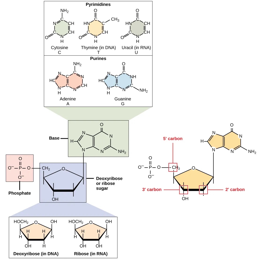
Figure 1:The components of a nucleotide. Credits: CC BY 4.0 Clark et al. (2018).
The bases can be divided into two categories: purines (with a double ring structure) and pyrimidines (with a single ring structure) (Figure 1). DNA contains A, T, C, and G; whereas RNA contains A, U, C, and G.
The DNA double helix
The DNA molecule is a polymer of deoxyribonucleotides and forms a right-handed double helix. The sugar and phosphate are on the outside forming the helix’s backbone and the bases are stacked in the interior and bind each other by hydrogen bonds. Thereby A pairs with T via two hydrogen bonds and C pairs with G via three hydrogen bonds, they are complementary bases. These pairings are also called Watson-Crick base-pairing, named after the discoverers of DNA.
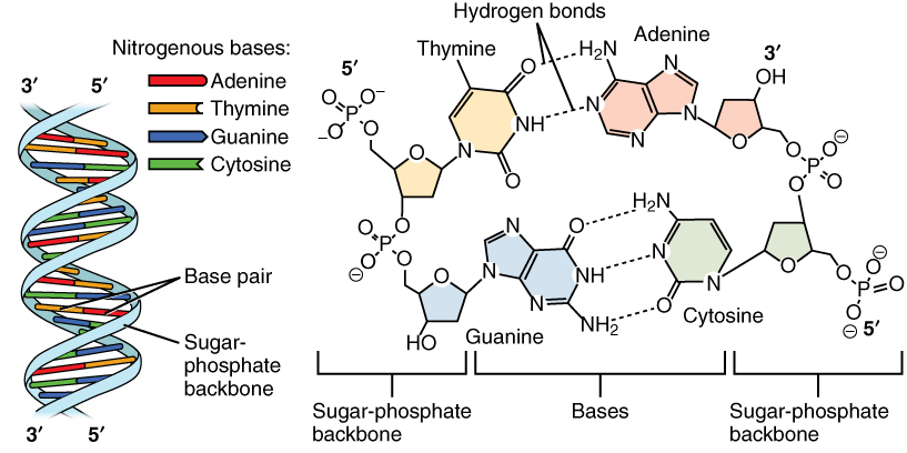
Figure 2:The DNA structure. Credits: CC BY 3.0 OpenStax College (2013).
The two strands of the helix run in opposite directions, also called anti-parallel, i.e., one goes from 5’ to 3’ and the other from 3’ to 5’ (Figure 2). The nucleotide sequence is typically written in 5’ to 3’ direction. Due to the complementarity, the base sequence of a strand can be deduced from the base sequence from the other strand. This is called the reverse complement. For example, the reverse complement of AAGT is ACTT, where both strands are given in 5’ to 3’ direction.
DNA replication
As the two DNA strands are only connected via hydrogen bonds, they can be separated relatively easily, for example during DNA replication (Figure 3). The separated strands each serve as a template on which a new complementary strand is synthesized by the enzyme DNA polymerase in 5’ to 3’ direction. This mode of replication is called semiconservative.
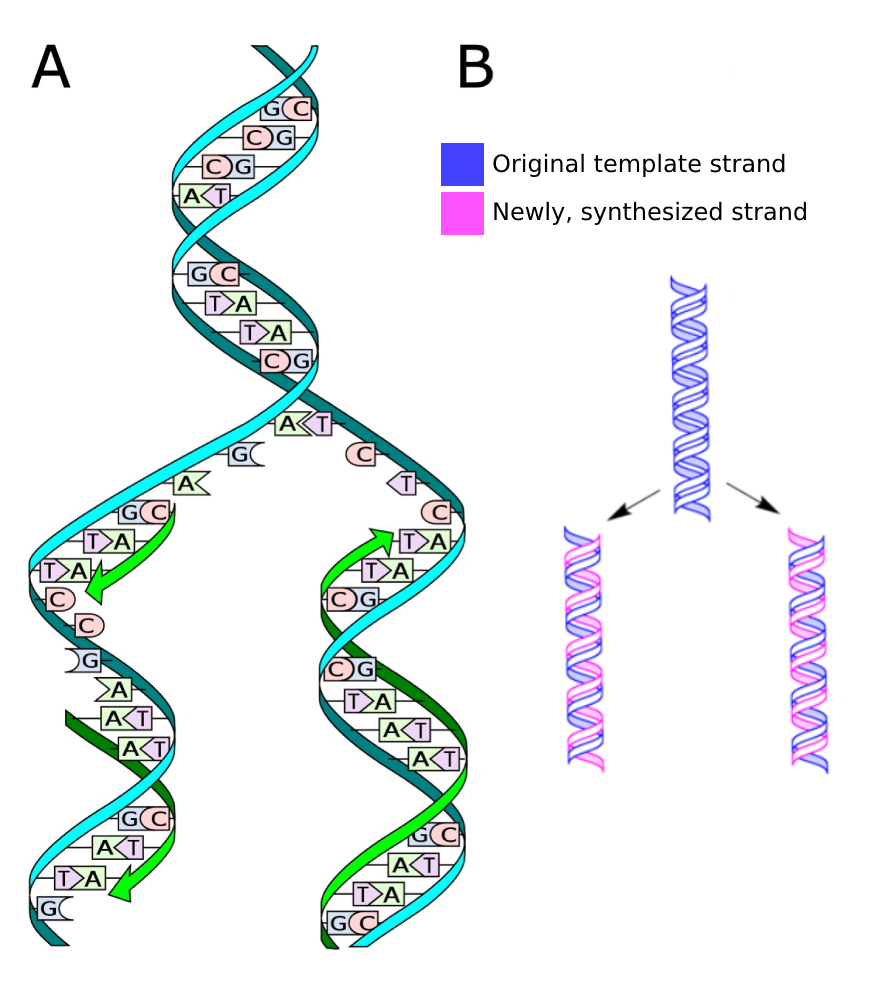
Figure 3:A) The process of DNA replication. Credits: CC0 1.0 Ball (2013). B) Semiconservative DNA replication, where the two copies each contain one original strand and one new strand. Credits: CC0 1.0 modified from Koch (2009).
The error rate of DNA replication is remarkably low, about one erroneous base in 109 bases. This property preserves the genetic information during cell division, and also over generations. It also leads to mutations over evolutionary time (Figure 4), as we will see later (Substitutions).
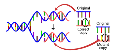
Figure 4:A DNA mutation that occurs during replication. Credits: BY-NC-SA 4.0 UC Museum of Paleontology (2020).
RNA, transcription, and splicing
During Transcription, RNA polymerase reads the template strand (also called noncoding strand) in the 3’ to 5’ direction (Figure 5). This produces an RNA molecule from 5’ to 3’, which is a copy of the coding strand. During transcription thymine is replaced by uracil. In contrast to DNA, RNA does not form a stable double helix. RNA is mainly single stranded, but most RNAs show intramolecular base pairing between complementary bases.
There are four major types of RNA:
- Messenger RNA (mRNA): RNA molecules that will later be translated into proteins and therefore serve as a ‘messenger’ in protein production.
- Ribosomal RNA (rRNA): the primary component of ribosomes (the ‘powerplants’ of a cell).
- Transfer RNA (tRNA): functions as ‘adapter molecule’ that serve as the physical link between mRNA and the amino acid sequence of a protein during translation.
- MicroRNA (miRNA): non-coding RNA molecules of 21-23 nucleotides involved in RNA silencing and post-transcriptional regulation of Gene expression.
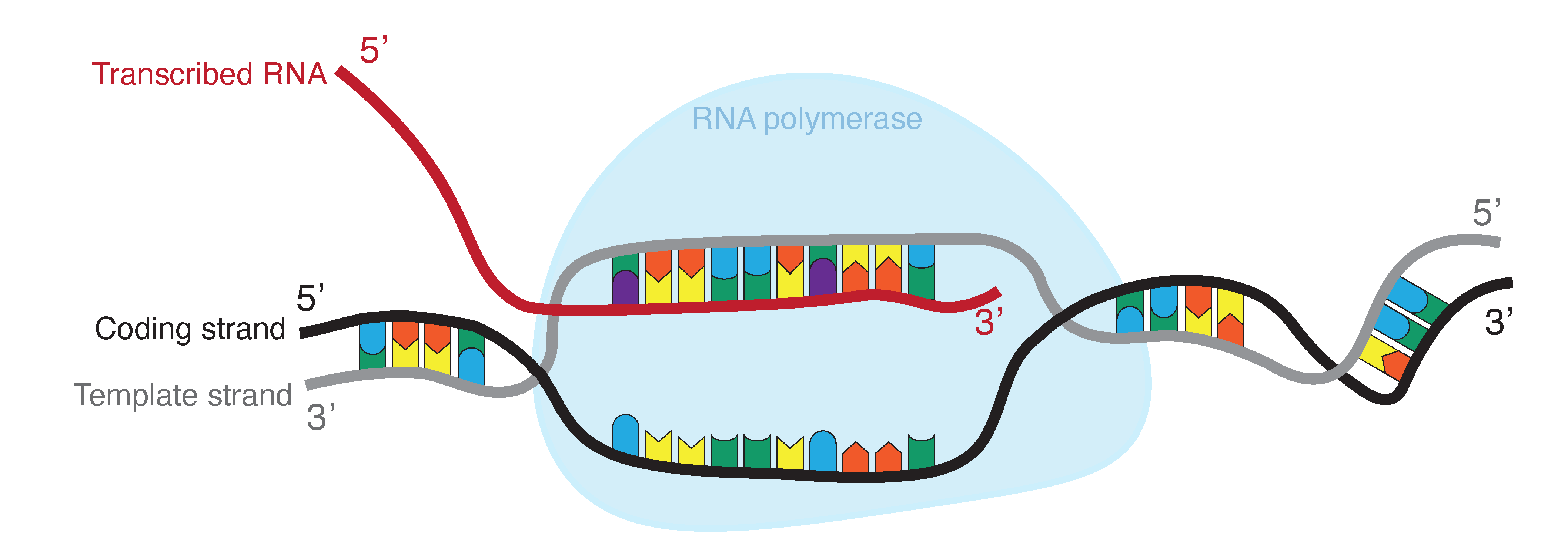
Figure 5:RNA is produced by transcribing DNA: as such, it is a direct copy of the information contained in the DNA. Where DNA contains thymine (T, indicated in blue), RNA contains uracil (U, indicated in purple). Credits: CC BY-NC 4.0 Ridder et al. (2024).
In eukaryotes, precursor mRNA molecules undergo various postprocessing steps to produce mature mRNA molecules. To stabilize the mRNA, the 5’ end of the molecule is capped with a modified guanine nucleotide (more specifically, a 7-methylguanylate) and the 3’ end is extended with a long stretch of adenine nucleotides (known as poly-adenylation). In addition, many eukaryotic mRNA molecules undergo Splicing. During RNA splicing, the spliceosome protein complex removes introns: specific non-coding parts of an mRNA molecule that are not used during translation (Figure 6), to create mature mRNA. Most introns are characterized by a GU and AG dinucleotide motif in the 5’ and 3’ end respectively.
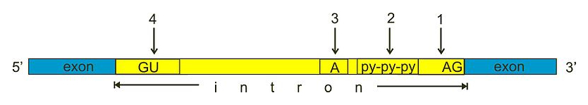
Figure 6:During splicing, introns are removed from precursor mRNA moleculus to create mature mRNA. Most introns contain recognition sequences for the spliceosome and produce specific secondary structures that improve splicing efficiency: (1) 3’ splice site, (2) poly pyrimidine tract, (3) branch site, (4) 5’ splice site’. Credits: CC0 1.0 miguelferig (2011).
Translation
During protein Translation, ribosomes synthesize polypeptides from messenger RNA (mRNA) (Figure 7). During this process tRNAs decode the information on the RNA into amino acids, where a codon consisting of three nucleotides encodes the information for one amino acid.
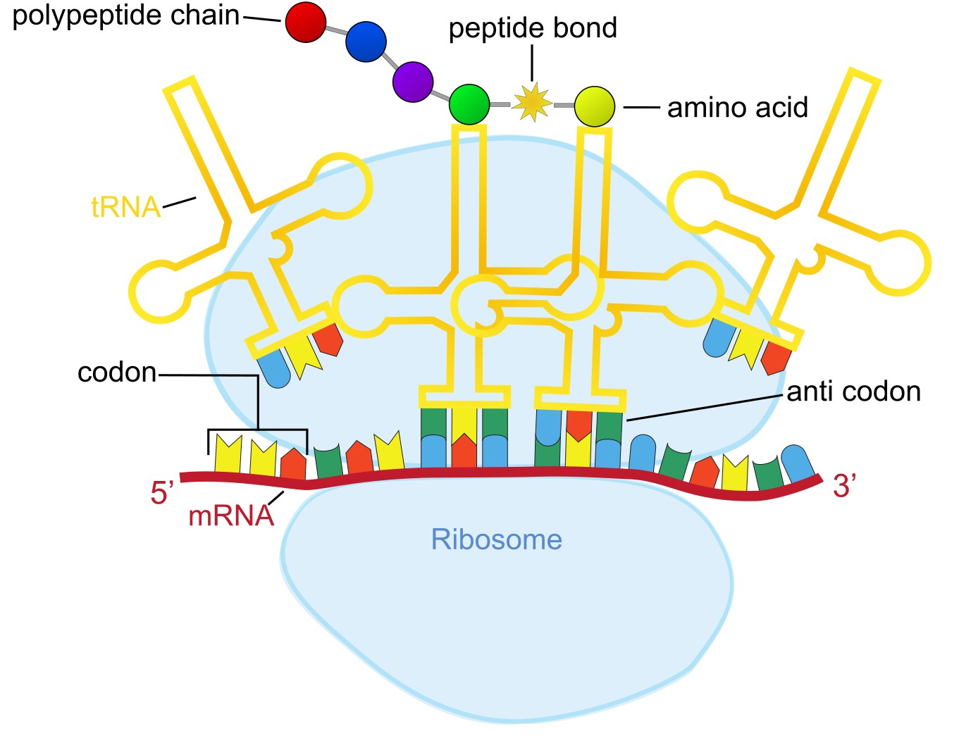
Figure 7:The translation process, where ribosomes with tRNA molecules “read” codons on the mRNA using anticodons, which then get translated into their corresponding amino acids. These amino acids are linked together by peptide bonds to form a polypeptide chain. Credits: CC BY-NC 4.0 Ridder et al. (2024).
The genetic code
The genetic code shows the correspondence between codons and amino acids (Figure 8). Since 64 possible codons code for 20 different amino acids, the genetic code is degenerate, i.e., most amino acids are specified by more than one codon. Thus, the codons encoding one particular amino acid may differ in one or two of their positions. You can notice in Figure 8 that the third codon position often differs between codons for the same amino acid. As a result of the code degeneracy, the protein sequence can be deduced from the DNA or RNA sequence but not vice versa.
There are three codons that do not encode for an amino acid, but instead signal the end of the protein sequence, called stop codons. Furthermore, translation generally starts with the start codon AUG encoding methionine. More information of how protein information is encoded in genomes can be found in the section on genome annotation.
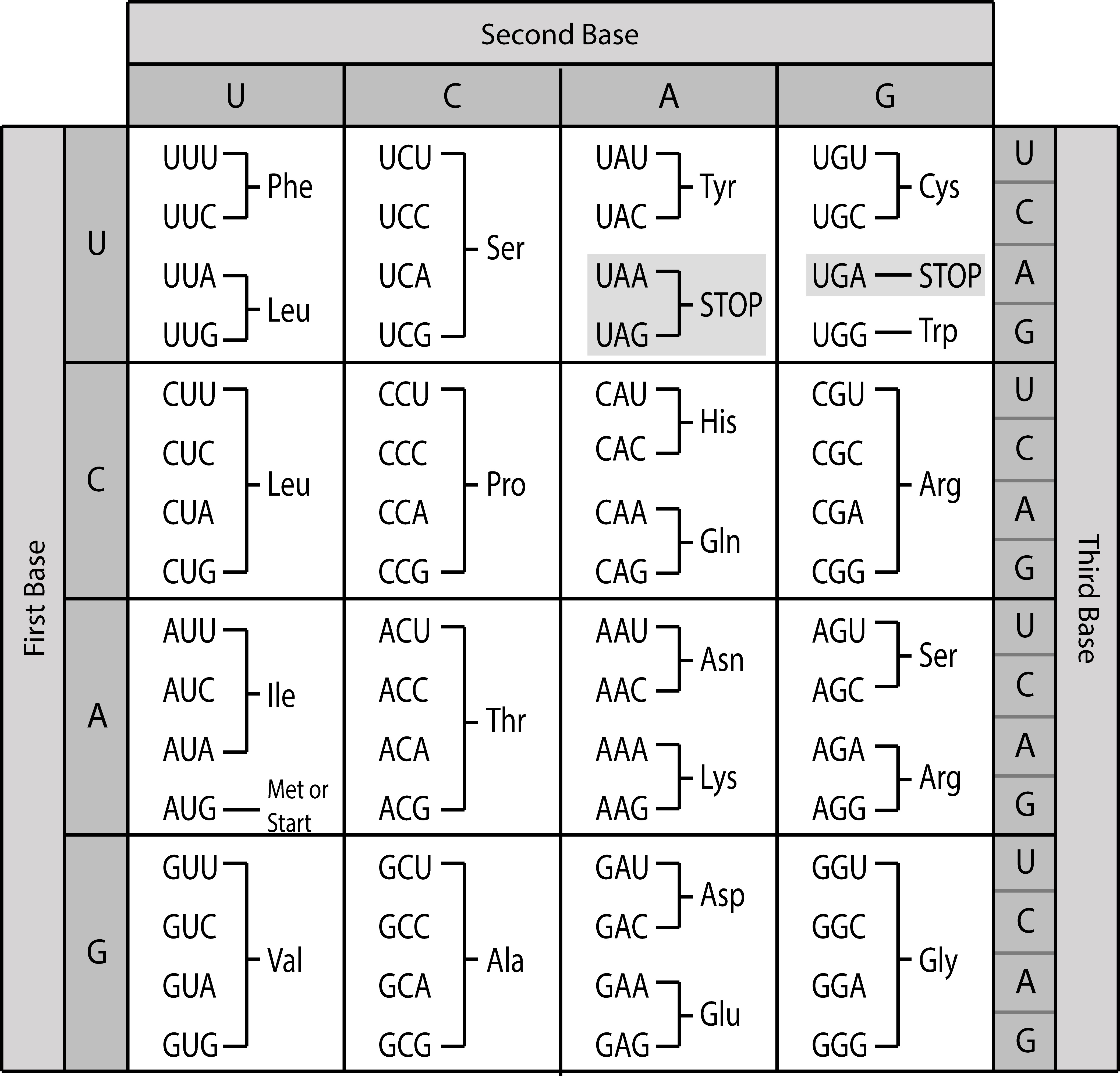
Figure 8:The universal genetic code. Note that exceptions to this code exist, for example the vertebrate mitochondrial code. Credits: CC BY 4.0 Greenwood (2018).
The central dogma of molecular biology
According to the central dogma of molecular biology, the flow of genetic information is essentially in one direction: from DNA via RNA to proteins (Figure 9). Nevertheless, there are also genes that do not code for proteins, but where functional RNA is the end product. Furthermore, mobile genetic elements and viruses can encode reverse transcriptases (which can synthesize DNA from an RNA template) or RNA dependent RNA polymerases (which can replicate RNA).
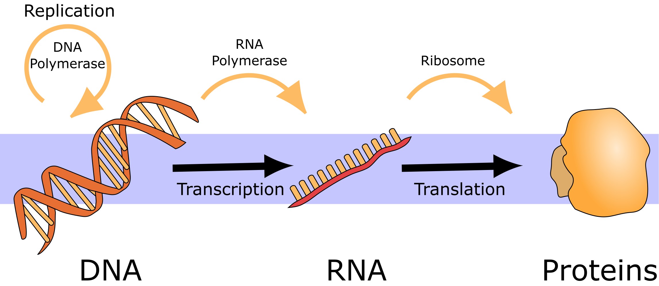
Figure 9:The central dogma of molecular biology. Credits: CC0 1.0 modified from Squidonius (2008).
Proteins
Proteins are large, complex macromolecules that play many important roles in the body. They are critical to most of the work done by cells and are required for the structure, function and regulation of the body’s tissues and organs. The basic building blocks of proteins are amino acids.
Amino acids
An amino acid contains a central carbon atom (called α-carbon, or Cα) (Figure 10). The α-carbon is bound to an amino group (NH2), a carboxyl group (COOH), and a hydrogen atom. In addition, each amino acid has a specific residue (R) group.
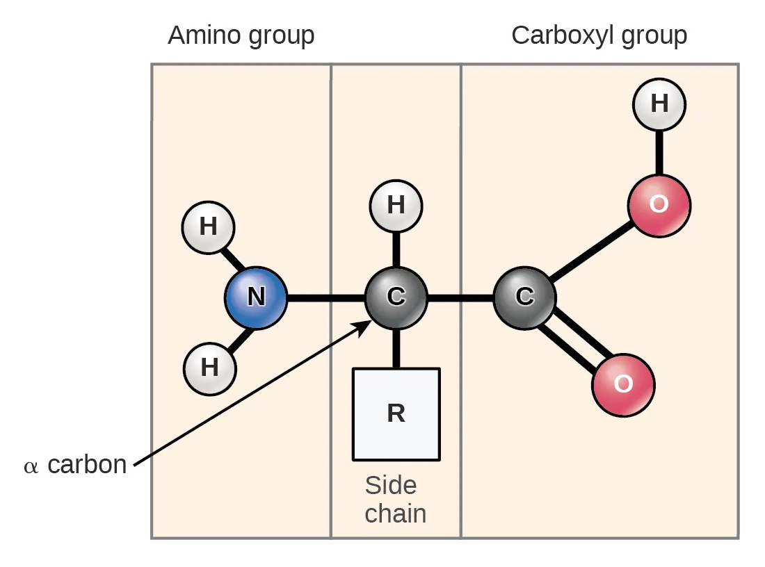
Figure 10:The structure of an amino acid. Four elements are connected to the α-carbon: an amino group, a hydrogen atom, a carboxyl group, and a side chain (R group). Credits: CC BY 4.0 Clark et al. (2018).
Table 1:Amino acids and their abbreviations and basic properties
| Amino acid | Three-letter code | One-letter code | Property |
|---|---|---|---|
| Arginine | Arg | R | Positively charged |
| Histidine | His | H | Positively charged |
| Lysine | Lys | K | Positively charged |
| Aspartic acid | Asp | D | Negatively charged |
| Glutamic acid | Glu | E | Negatively charged |
| Serine | Ser | S | Polar uncharged |
| Threonine | Thr | T | Polar uncharged |
| Asparagine | Asn | N | Polar uncharged |
| Glutamine | Gln | Q | Polar uncharged |
| Alanine | Ala | A | Hydrophobic |
| Valine | Val | V | Hydrophobic |
| Isoleucine | Ile | I | Hydrophobic |
| Leucine | Leu | L | Hydrophobic |
| Methionine | Met | M | Hydrophobic |
| Phenylalanine | Phe | F | Hydrophobic and aromatic |
| Tyrosine | Tyr | Y | Hydrophobic and aromatic |
| Trypotophan | Trp | W | Hydrophobic and aromatic |
| Glycine | Gly | G | Special (only H as side chain) |
| Proline | Pro | P | Special (side chain bound to backbone nitrogen) |
| Cysteine | Cys | C | Special (forms disulfide bonds) |
Some amino acids have non-polar side chains, and these are generally hydrophobic, i.e., water molecules cannot form hydrogen bonds with these molecules. Thus, they can often be found in the interior of proteins together with other hydrophobic amino acids. Aromatic amino acids contain aromatic rings, and often stabilize folded protein structures.
In contrast, the charged and the polar amino acids are hydrophilic, i.e., water molecules can form hydrogen bonds with these molecules. They can often be found on the surface of proteins or in the interior, when they can interact with another oppositely charged amino acid. Positively charged amino acids, are also called basic amino acids and negatively charged amino acids are also called acidic amino acids.
Although amino acids can be classified into these groups based on their properties, some amino acids stand out. The smallest amino acid is glycine, which provides great flexibility due to its small size. In contrast, proline is an amino acid, where the side chain is bonded to the backbone nitrogen atom, which makes it very rigid. Finally, one cysteine amino acid can form a disulfide bridge with another cysteine.
Protein structure
A protein is made up of one or more long, folded chains of amino acids (each called a polypeptide). The 3D structure of a protein is also called its conformation. The protein conformation is described on four levels - primary to quaternary structure (Figure 11).
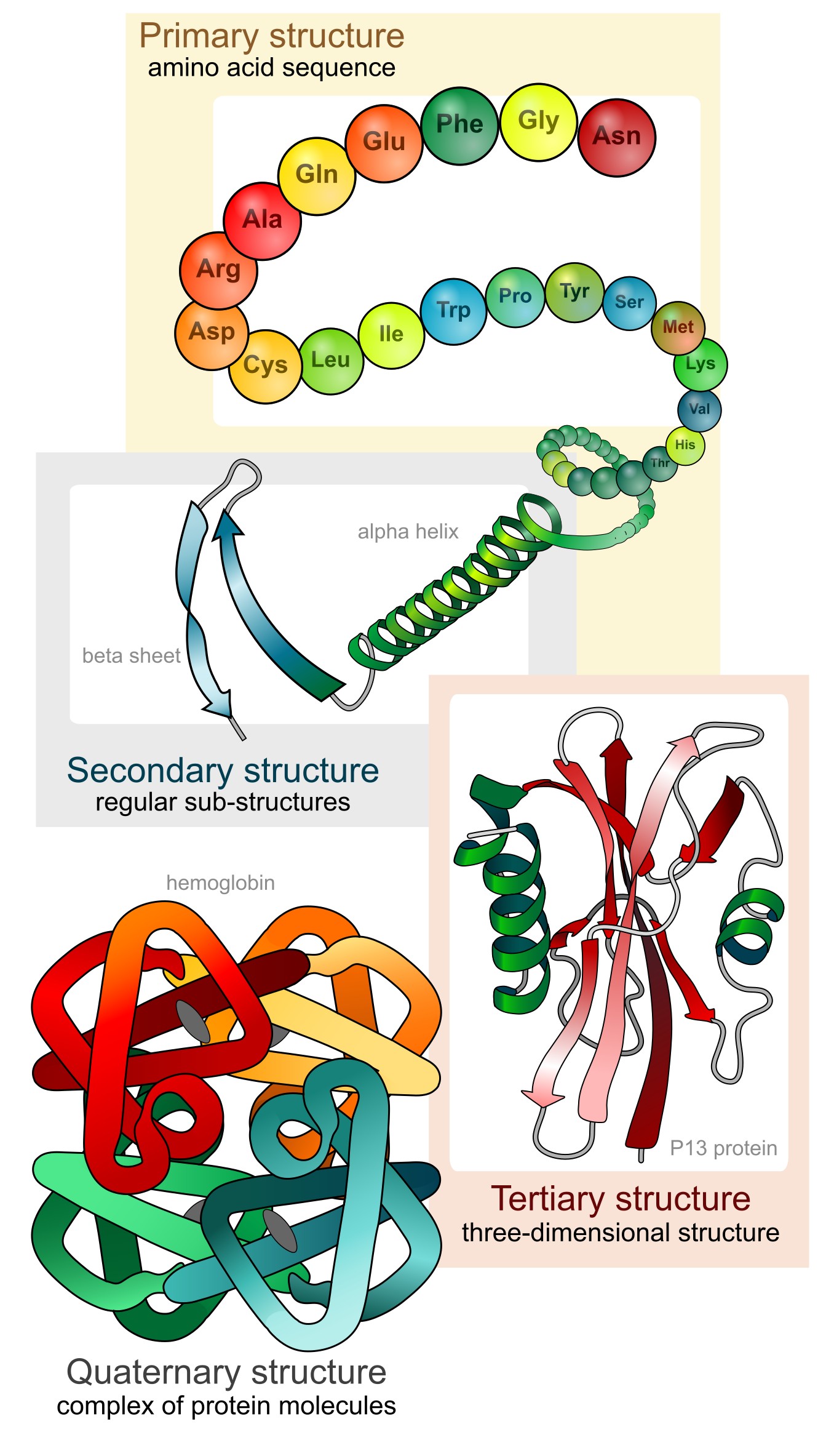
Figure 11:The four levels of protein structure. Credits: CC0 1.0 LadyofHats (2008).
The structure of a protein is critical for its function. For example, in an enzyme, the active site must be in the correct structure to be able to bind the substrate. Other proteins might bind proteins (and influence their activity) or bind DNA (and regulate gene expression). Additionally, some proteins are secreted from the cell or might function within the cell membrane. Finally, proteins are often modified after protein synthesis (see Translation), called post-translational modification. These modifications can be important for protein function.
Primary structure
In a protein, amino acids are connected by covalent bonds, called peptide bonds. A peptide bond connects one amino acid’s carboxyl group and the next amino acid’s amino group (Figure 12). The sequence of amino acids linked by peptide bonds is called the primary structure. The protein sequence is determined by the gene sequence encoding the protein. The continuous chain of atoms along the protein is also called the backbone, it consists of the three backbone atoms (nitrogen, Cα, carbon).
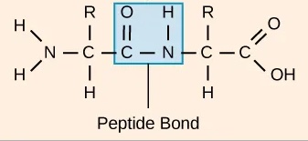
Figure 12:A peptide bond connecting two amino acids. Credits: CC BY 4.0 Clark et al. (2018).
Each protein has a free amino group on one end, called the N terminus. The other end has a free carboxyl group, called the C terminus.
Secondary structure
Secondary structures are local conformations in the protein that are stabilized by hydrogen bonds between backbone atoms. We distinguish the regular helices (i.e., alpha helix - α-helix) and sheet structures (i.e., beta sheet - β-sheet) (Figure 13) and irregular turns.
α-helices are stabilized by hydrogen bonds between the oxygen atom in the C group in one amino acid, and the hydrogen in the N group of the amino acids that is four amino acids farther along the chain. Every helical turn has 3.6 amino acids residues and the side chains stick out of the helix.
β-pleated sheets (short: β-sheets) consist of β-strands, where the R groups extend above and below the strands. The strands have a direction determined by the N- and C-terminus of the protein and are usually depicted as an arrow pointing towards the C-terminus. Depending on the direction, strands can align parallel or antiparallel to each other.
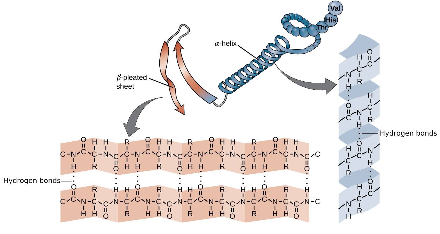
Figure 13:α-helices and β-sheets are stablized by hydrogen bonds (the dotted lines) between the backbone of proteins, i.e., the side chains are not involved. The hydrogen bonds form between the oxygen atom in the C group in one amino acid and the hydrogen in the N group. Credits: CC BY 4.0 modified from OpenStax College (n.d.).
Turns are short secondary structure elements that are stabilized by hydrogen bonds between amino acids that are 1 to 5 peptide bonds away. The most common form are β-turns, which connect antiparallel β-strands.
The peptide bond is very rigid and planar, i.e., it cannot rotate to form the elements of protein structure. However, the N-Cα and the Cα-C bonds can freely rotate, being only limited by the size and properties of the R-groups. The 3D shape of the polypeptide backbone is thus determined by two torsion angles: phi (φ) between N and Cα and psi (ψ) between Cα and C (Figure 14A). Although φ and ψ can rotate in principle, steric hindrance prevents certain combinations of angles, i.e., the bulkiness of the R-groups restricts the possible conformations. Thus, certain combinations of φ and ψ are preferred. We can plot the combinations of φ and ψ in a protein, in a so-called Ramachandran plot (Figure 14B).
The regular secondary structure elements (α-helix and β-sheet) contain consecutive amino acids with similar (φ,ψ) values. These regions are typically highly populated in a Ramachandran plot. Thus, the Ramachandran plot can be used to assess how plausible a predicted protein structure is.
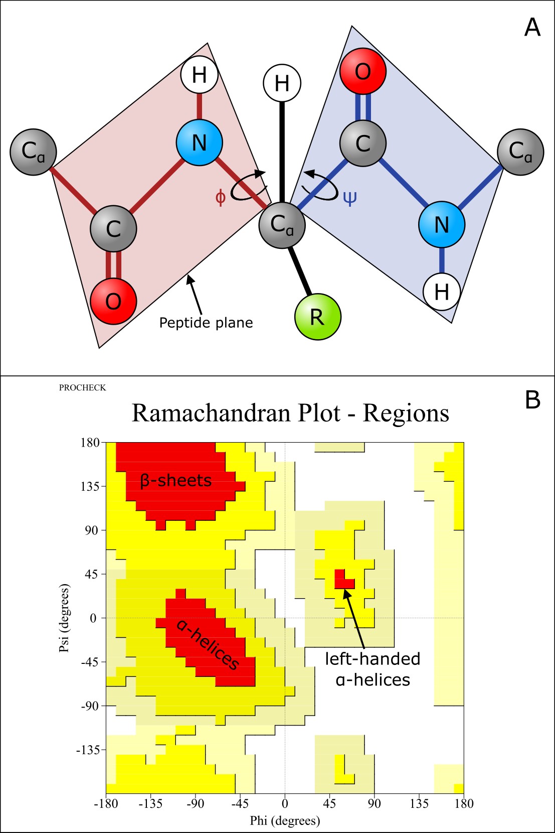
Figure 14:A) The φ, and ψ torsion angles of a polypeptide chain. Credits: CC BY-NC 4.0 Ridder et al. (2024). B) A typical Ramachandran plot. The red regions marked do not have any steric hindrance, yellow areas represent conformations that have steric hindrance, light yellow areas represent conformations that are generally sterically unfavorable, and white areas do not have any allowed conformations. Credits: Ramachandran plot modified from PROCHECK Laskowski et al. (1993).
Tertiary structure
The tertiary structure of a protein describes the complete folding of an entire polypeptide chain. In contrast to the secondary structure, the tertiary structure of a protein involves interactions between the amino acid’s side chains that can occur at short-range and long-range (Figure 15). Thus, the chemical properties of the amino acids are very important for the tertiary structure. Different types of interactions stabilize the tertiary structure:
- Hydrogen bonds involving polar amino acids.
- Ionic bonds between positively and negatively charged amino acids.
- Hydrophobic R groups that tend to lie in the protein’s interior, stabilized by hydrophobic interactions.
- Disulfide bonds (i.e., covalent bonds between cysteines).
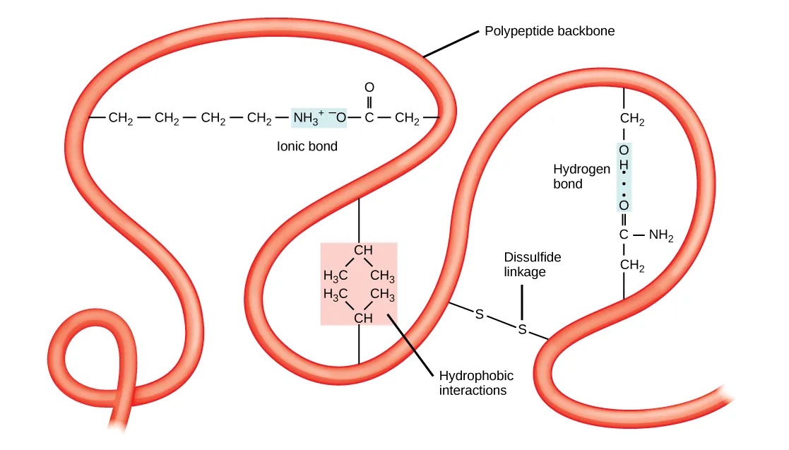
Figure 15:Chemical interactions that stabilize the tertiary structure of proteins. Credits: CC BY 4.0 Clark et al. (2018).
When studying many different protein structures, various reoccurring substructures can be observed. These so-called Domains are distinct functional and/or structural units in a protein and are typically 50 to 350 amino acids long. Usually, a domain is responsible for a particular function or interaction, contributing to the overall role of a protein. A domain can exist in different contexts with other domains (Figure 16). In a multidomain protein, each domain folds independently of the others.
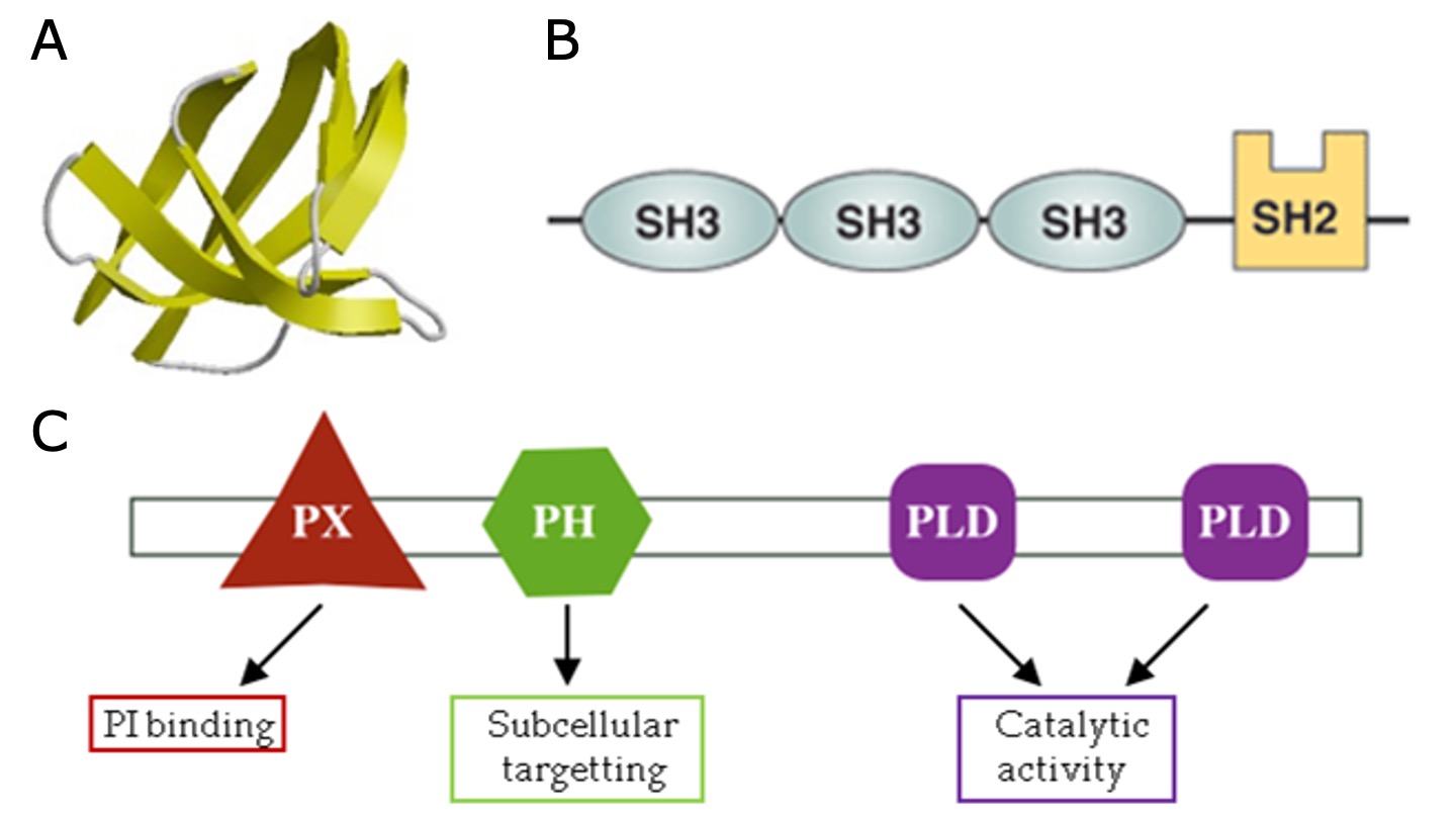
Figure 16:A) Example of an Src homology 3 (SH3) domain that is involved in protein-protein interaction. SH3 domains occur in a diverse range of proteins with different functions. B) The cytoplasmic protein Nck contains multiple SH3 domains. C) Domain composition of phospholipase D1, which has multiple functional domains that contribute to its overall function. Credits: CC BY 4.0 Sangrador (2023).
Quaternary structure
Finally, individual folded polypeptides can interact to form protein complexes, also called quaternary structures. The quaternary structure is stabilized by the same types of interactions as the tertiary structure. The difference is that the amino acids involved belong to different polypeptides.
Many functional proteins are composed of multiple subunits, they are also called oligomers (Figure 17). The subunits can originate from the same protein sequence (called a homomer) or from different sequences (called a heteromer). Proteins consisting of two subunits are also called dimer.
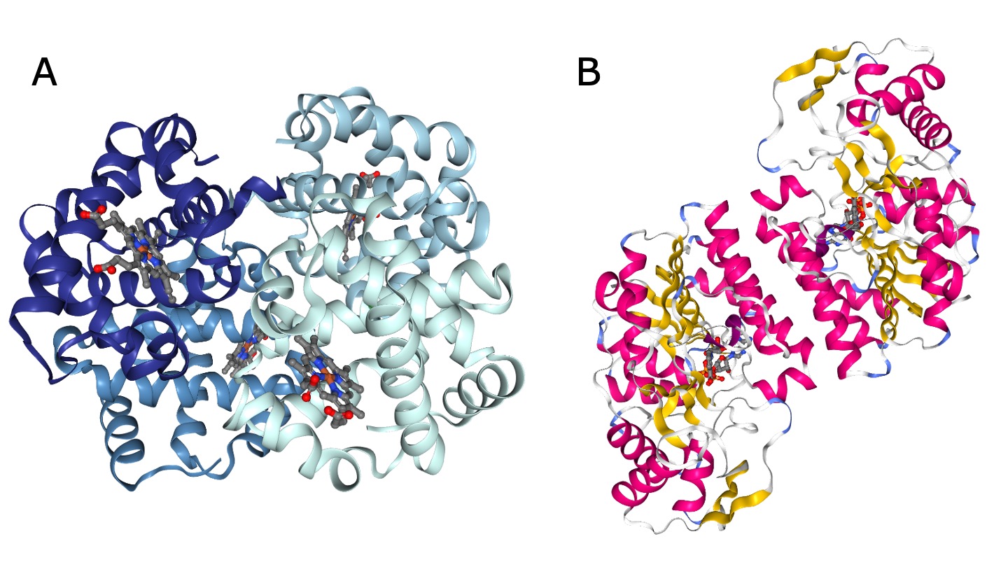
Figure 17:Examples of oligomers. A) Myoglobin, a heteromer of four subunits (PDB structure 1HV4 colored by chain). Credits: Berman et al. (2000)Liang et al. (2001)Rose et al. (2018). B) UDP-galactose 4-epimerase, a homodimer (PDB structure 1EK5 colored by secondary structure). Credits: Berman et al. (2000)Thoden et al. (2000)Rose et al. (2018).
Substitutions
Mutations in the gene sequence can lead to changes in the primary structure of the protein, e.g., a substitution of one amino acid by a different one. Often, such substitutions still lead to highly similar protein structures that perform a similar or even the same function, especially when the exchanged amino acids have similar chemical properties. Nevertheless, single amino acid substitutions can have severe consequences. A prominent example is sickle cell anemia, where a substitution of glutamic acid to valine in hemoglobin β results in a structural change that leads to a distortion in red blood cells (Figure 18).
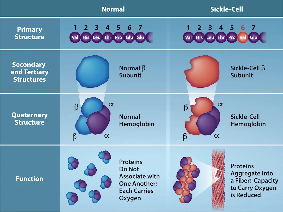
Figure 18:Consequences of a substitution in hemoglobin β resulting in sickle cell anemia. Credits: Rao, A., Tag, A. Ryan, K. and Fletcher, S. Department of Biology, Texas A&M University.
Visualization
There are many styles to view protein molecular structures. Some styles focus on detailed chemical structure, others are targeted at the protein surface. For some examples see Figure 19.
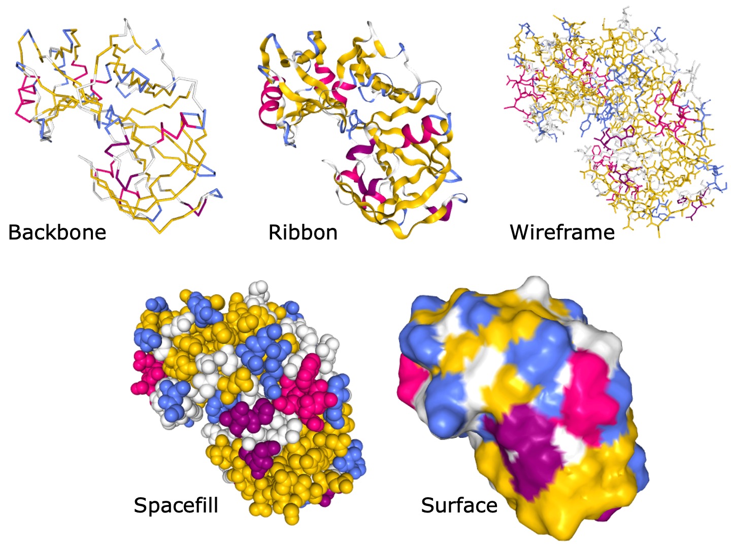
Figure 19:Different representations of the PDB structure 5PEP generated with NGL. Credits: Berman et al. (2000)Cooper et al. (1990)Rose et al. (2018).
Genome annotation
Annotation of genomes is the process of deciphering what information is encoded in an organism’s DNA. It is an ongoing effort in organisms with known genome sequences. Even moreso, genome annotation is a critical step in acquiring biological insights from newly sequenced genomes. Given the large size of any genome, automated procedures are used to identify various genomic elements such as genes, regulatory regions, transposable elements, or other non-coding elements. Each of these bioinformatic procedures typically focuses on identifying one type of element, and as such a complete genome annotation project can be thought of as a pipeline of various procedures. The following section describes the most common steps in genome annotation.
Repeat masking
Repeat masking involves the identification and masking (hiding) of repetitive sequences within a genome. It is an essential first step in annotating most genomes because repetitive sequences can pose significant challenges in genome annotation. Masking repeats generally improves:
- Accuracy: repetitive elements can be mistakenly annotated as genes or other functional elements, leading to inaccurate predictions and interpretations of the genome.
- Computational efficiency: identifying and processing repetitive sequences can be computationally intensive. However, masking these repetitive regions reduces the computation time of all downstream analyses.
- Biological relevance: repetitive sequences are usually not involved in the coding of proteins of interest. Therefore, focusing on non-repetitive regions is a smart choice in understanding the genes and regulatory elements that drive biological processes.
Most repeat masking workflows work by first compiling (or using a precompiled) ‘repeat library’: a collection of known repetitive elements that have previously been characterized. Subsequently, the genome to be annotated is compared against this repeat library using various computational algorithms, such as (specifically configured versions of) BLAST or RepeatMasker. When a match is found, the corresponding region in the genome is ‘masked’ or annotated as a repetitive element. This means that these regions are excluded from further analysis or labeled as repetitive.
Gene prediction
The process of finding protein coding genes differs between prokaryotic and eukaryotic genomes. In both cases the aim is to find open reading frames (ORFs): contiguous stretches of nucleotides that encode proteins. More specifically, an ORF starts with a start codon, ends with a stop codon, and it’s length is a multiple of three (Refer to the genetic code in Figure 8). Since RNA splicing (Figure 6) is almost absent in prokaryotic genomes, prokaryotic ORFs can be found directly in the genomic DNA. As a result, simply enumerating all possible ORFs in a genome is a common step in prokaryotic genome annotation. In contrast, ORFs in eukaryotic genomes are found on mature mRNAs. As such, all eukaryotic gene prediction methods take splicing into account, thereby greatly increasing their computational complexity. Both prokaryotic and eukaryotic gene prediction typically can be classified as either evidence based prediction or ab initio prediction, both will be explained below.
Evidence based prediction
This data-driven approach uses existing and newly generated data to get hints on what regions of a genome encode genes. Depending on the type of data, these predictions have more or less predictive power. Some commonly used evidence types are:
- RNA-sequencing data: the most direct form of evidence for what regions of the genome are transcribed. As such, RNA-sequencing (often abbreviated to RNA-seq) ‘reads’ often provide the best form of evidence in identifying splice sites in eukaryotes. Note that not all transcribed RNA will be translated into proteins, and that therefore not all RNA-sequencing reads are evidence for protein coding genes. Distinguishing between protein-coding and non-coding RNA is not always trivial.
- Homology evidence: Aligning DNA or protein sequences of known genes (from other organisms) is valuable evidence in finding coding regions of the genome. Due to the redundancy in the genetic code, it is not trivial to correctly identify splice sites when aligning protein sequences to a genome. Homology evidence from closely related organisms leads to higher quality predictions than evidence from distantly related organisms.
- Whole-genome alignments: this approach uses the annotated genome of a closely related organism to directly identify coding regions in a novel genome. For example: whole-genome alignment of mouse and human genomes reveals that large parts of mouse chromosome 2 are homologous to human chromosome 20. The alignment procedure results in a direct 1-to-1 mapping of mouse and human genome coordinates, and as such annotation coordinates can be transferred between genomes.
Ab initio prediction
Ab initio (latin): from first principles, from the beginning
These methods rely on statistics to learn a predictive model from a known annotated genome. Various forms of ab initio models exist, and whereas implementation details differ, most follow a similar line of reasoning. For now, we will stick to a high level description. All ab initio models scan through a DNA sequence and at each position give a score for a specific type of annotation. In addition, they often take the genomic context of a specific position into account. For example, the probability of a protein-coding annotation on a nucleotide A is high when the next two observed nucleotides are T and G, producing the ATG start-codon methionine. In addition, most methods also take the predicted annotation of the genomic context into account. For example: the probibility that ATG actually codes for a start codon is much higher if we can also predict an in-frame stop codon. In eukaryotic genome prediction these models become quite complex because they have to include splice sites in all three reading frames. How exactly a model decides what annotation score to give to which nucleotide is part of the model architecture and parameterization. In all cases, the model parameters are chosen to accurately reproduce a known genome annotation. If sufficient data is used to learn the model parameters, it is assumed that these models can be used to predict annotations on novel genome sequences. Like homology-based prediction, this model-based approach works best for closely related organisms. In the past, almost all ab initio prediction methods were formulated as hidden Markov models (HMMs) (see Note 1.5). Examples of tools implementing HMM based ab initio prediction are SNAP, GeneMark, and Augustus. With the availability of more high quality data (genome sequences and accompanying annotations), approaches based on deep learning and generative AI have proven to frequently perform better than HMM based approaches.
Evidence/prediction integration
From the previous sections it has now become clear there are several ways of predicting what the genes in a genome look like. Since these various approaches almost never agree exactly in their predictions, a final step in genome annotation is evidence and prediction integration. Typically a weighted consensus approach is used: each individual source of evidence is given a weight representing how much it should influence the final decision, after which a majority vote decides what the annotation should look like. Typically RNA-seq evidence gets a high weight, and various forms of homology evidence can be weighted depending on how closely related they are to the genome of interest.
Functional annotation
So far, all described steps in the genome annotation process have dealt with what genes look like on a structural level. To gain biological insight, the next step is to assign functional annotations to the predicted genes. This functional annotation step consists of using various sequence alignment and search tools to find sequences with a known function/description and to transfer the information of the known gene to the predicted gene. Several databases of high-quality known functions are often used, which are described in more detail in the next section of this chapter. In Chapter 2 we will learn about approaches how to search these databases efficiently.
Databases
Introduction
Databases are at the core of bioinformatics. In all analyses, we integrate pre-existing data and we need to access this data. The journal Nucleic Acids Research publishes an entire issue in the beginning of each year on new and updated databases. The list of these databases can also be accessed online.
Computer scientists have developed different kinds of databases. One example are relational databases, which can be queried by SQL (structured query language) and which perform well for data that is processed computationally. Another example are XML (extended markup language) databases which store data in specified well-structured XML files. Nevertheless, most databases for biological sequence data use flat file databases, where the data is saved in structured text files. This data can be manipulated in a text editor without requiring an additional program for database management, and they can be easily exchanged between scientists. On the downside, searching them has a lower performance. This is why they are often indexed, i.e., they contain an index of keywords, similar to a glossary in a book.
Depending on the kind of data included, we distinguish different kinds of biological databases:
- Primary databases contain primary sequence information from experimentally derived data that is directly submitted by the scientists that generated the data.
- Secondary databases provide the results of analyses of the information in primary databases.
Each entry in a database has a unique accession number. This number is permanent and provides an unambiguous way to link to the entry. The information that the accession refers to should not change. To still allow updates to an entry, the accession number can contain a version, usually after a dot. For example, NC_003070.9 is the latest version (version 9) for Arabidopsis thaliana chromosome 1 in RefSeq.
Database entries often link to each other via cross links.
GenBank
GenBank is a popular primary database for nucleotide sequences and is based at the NCBI (National Center for Biotechnology Information). A GenBank release usually occurs every two months and the most recent release from the 15th of December 2023 contains ~250 million sequences and additionally ~3.7 billion WGS (whole genome shotgun) records. The latter are genome assemblies or genomes that were not yet completed. The complete database is available for download via FTP, but the most convenient way to access individual entries is via the search on the GenBank website (Figure 23).
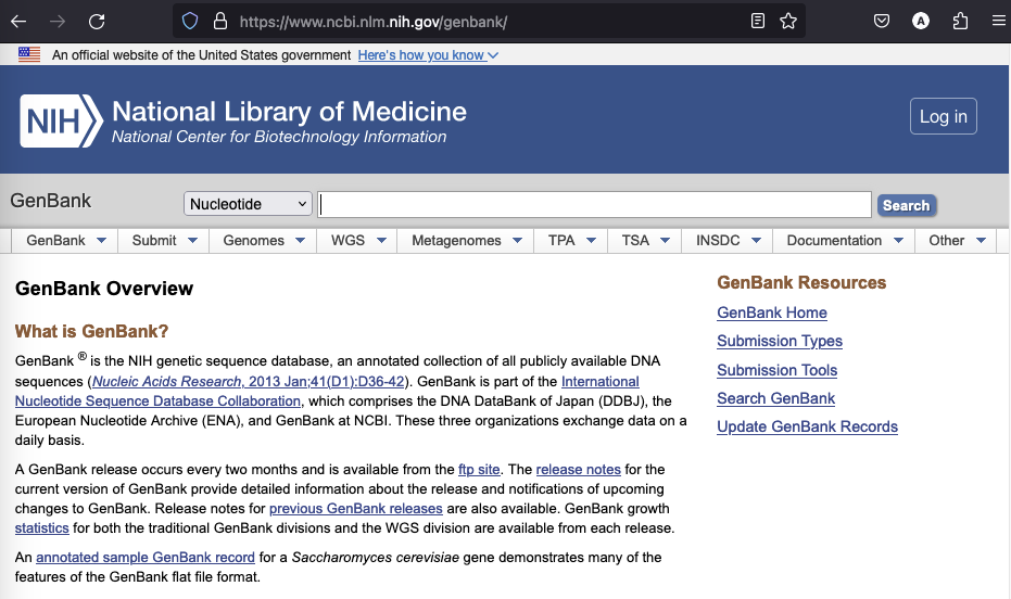
Figure 23:A screenshot of the GenBank website. Credits: Benson et al. (2012).
Since data is directly submitted to GenBank, the information for some loci can be highly redundant. The sequence records are owned by the original submitter and cannot be altered by someone else.
Genbank is part of the INSDC (International Nucleotide Sequence Database Collaboration). The other two member databases are ENA (European Nucleotide Archive) and DDBJ (DNA Data Bank of Japan). The data submitted to either database is exchanged daily, so all databases contain essentially the same information.
RefSeq
The Reference Sequence (RefSeq) collection is also hosted at NCBI and contains genomic DNA, transcripts, and proteins. The aim of RefSeq is to provide non-redundant, curated data. RefSeq genomes are copies of selected assembled genomes in GenBank. Additionally, transcript and protein records are generated by several processes:
- Computation via the eukaryotic or prokaryotic annotation pipeline.
- Manual curation.
- Transfer of information from annotated genomes in GenBank. In contrast to GenBank, RefSeq records are owned by NCBI and can be updated to maintain annotation. The current release is 231 from the 11th of July 2025 and contains ~418 million proteins from ~167,000 organisms.
The RefSeq accessions directly provide information on molecule types.
For example, NC_ accessions denote complete genomes, NP_ accessions denote proteins in one genome, and WP_ accessions denote proteins in multiple genomes.
UniProt
There is lots of information available for proteins, such as sequence information, domains, expression, or 3D structure. The aim of the Universal Protein Resource (UniProt) is to provide a comprehensive resource for proteins and their annotation. UniProt contains three databases (Figure 24):
- UniProt Knowledgebase (UniProtKB) - see below.
- UniProt Reference Clusters (UniRef - clusters of protein sequences at 100%, 90%, and 50% identity.
- UniProt Archive (UniParc - non-redundant archive of publicly available protein sequences seen across different databases.
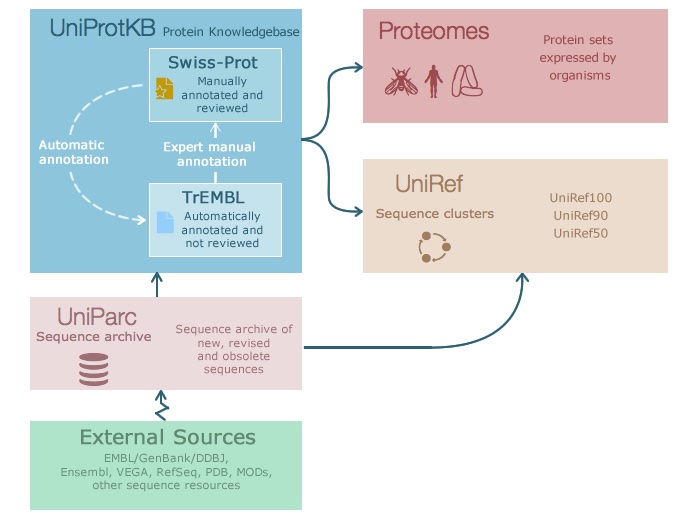
Figure 24:The information flow in Uniprot. Credits: CC BY-NC-ND 4.0 Leon & Pastor (2021).
UniProtKB is the central hub for functional information on proteins. For each protein it contains the core data (such as sequence, name, description, taxonomy, citation) and as much annotation information as possible. It contains many cross-references to other databases and is generally a very good starting point to find information on a protein.
UniProtKB consists of two sections:
- Swiss-Prot - manually-annotated records with information extracted from literature and curated computational analysis.
- TrEMBL - automatically annotated records that are not reviewed.
UniProtKB is updated every 8 weeks. The current release has ~570,000 entries in Swiss-Prot and ~250 million entries in TrEMBL.
Prosite
Prosite is a secondary database of protein domains, families, and functional sites. Some regions in protein families are more conserved than others because they are important for the structure or function of the protein. Prosite contains motifs and profiles specific for many protein families or domains. Searching motifs in new proteins can provide a first hint for protein function.
The current release of Prosite from the 18th of June 2025 contains 1311 patterns, 1403 profiles, and 1421 ProRule entries.
A Prosite pattern is typically 10 to 20 amino acids in length.
These short patterns are usually located in short well-conserved regions, such as catalytic sites in enzymes or binding sites.
A pattern is represented as a regular expression, where amino acids are separated by hyphens and x denotes any letter.
Repetitions can also be given as the number of repetitions in brackets.
For example, [AC]-x-V-x(4)-{ED} matches sequences that contain the following amino acid sequence: (Alanine or Cysteine)-any-Valine-any-any-any-any-(any but Glutamic acid or Aspartic acid).
Note that this representation is qualitative, a sequence either matches a pattern or it does not.
Patterns cannot deal with mismatches and are limited to exact matches to the pattern. Thus, they are not well suited to identify distant homologs. A Prosite profile is more general than a pattern and can also detect poorly conserved domains or families. They characterize protein domains over their entire length and do not just model the conserved parts. Profiles are estimated from multiple sequence alignments and we learn more about them in Chapter 2. For now, it is important to know that profiles model matches, insertions, and deletions. Importantly, profiles are quantitative representations, they will return a score how well the sequence fits to the profile. A threshold can be applied to get high-scoring profiles for a sequence. In contrast to patterns, a mismatch to a profile can be accepted if the rest of the sequence is highly similar to the profile. Profiles are well suited to model structure properties of a domain.
Notably, profiles cover the structural relationships of domains, but they might also score a sequence highly that lacks important functional residues. To include that information, ProRule contains additional information about Prosite profiles, such as the position of structurally or functionally important amino acids. ProRule is used to guide curated annotation of UniProtKB/Swiss-Prot.
InterPro
The Integrated Resource of Protein Families, Domains and Sites (InterPro) integrates 13 member databases (including Prosite and Pfam) into a comprehensive secondary database. Additionally, it provides annotation from other tools, for example to annotate signal peptides and transmembrane regions. It allows to identify functionally important domains and conserved sites in a sequence by simultaneously annotating it using the member databases. Interpro can be used to find out which protein family a sequence belongs to, or what its putative function is. Additionally, one InterPro entry can integrate entries from the member databases, if they represent the same biological entity, reducing redundancy. InterPro entries are also linked to Gene Ontology. They are curated before being released.
InterPro is updated every 8 weeks. The current release from the 19th of June 2025 contains ~49,000 entries, which represent different types:
As an example, look at the InterPro entry for the type 2 malate dehydrogenase protein family. The entry has a name (malate dehydrogenase, type 2) and accession (IPR010945). The contributing entries in member databases are shown on the right-hand side, with links to the individual member database entries. A descriptive abstract explains what these proteins are and what their function is. A set of GO terms is also provided, which describe the characteristics of the proteins matched by the entry.
You can get the InterPro annotation for a protein by running a new sequence search (Figure 25), or by by looking up its UniProt accession (Figure 26).
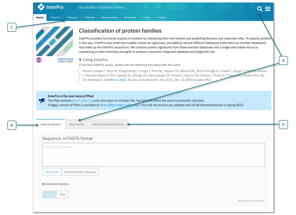
Figure 25:Search fields on the InterPro home page, showing text search field (A) and the sequence search (B) options, including ‘Advanced options’, where you can limit your search to member databases or sequence features of interest. Selecting the browse tab in the top menu (C) allows access to a browse search, (e.g., search for member database signature, InterPro entry type), see also Figure 26. You can also search for a particular domain architecture (D). Credits: Paysan-Lafosse et al. (2022).
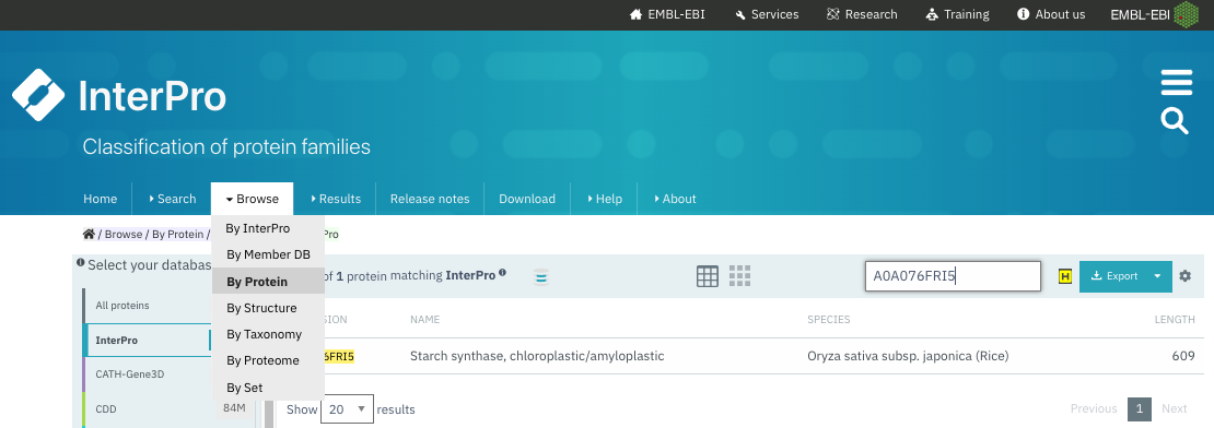
Figure 26:Browse the annotated proteins in Interpro and search for a UniProt accession. See resulting entry in (Figure 27). Credits: Paysan-Lafosse et al. (2022).
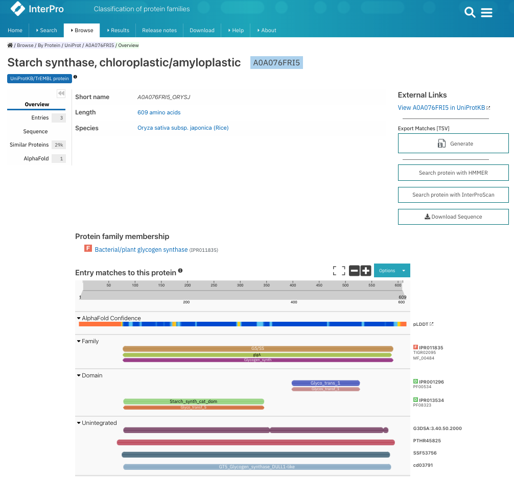
Figure 27:The result page when looking up UniProt accession A0A076FRI5 in InterPro. You can see the family and domain annotation and on the right the accessions in InterPro and in the member databases. You can click on each of these accessions to get to the entry information. Credits: Paysan-Lafosse et al. (2022).
You may have noticed a colored letter before each InterPro accession, e.g., F before IPR011835 or D before IPR001296 (Figure 27). These icons denote the different InterPro entry types:
- (Homologous) Superfamily - a large diverse family, usually with shared protein structure.
- Family - a group of proteins sharing a common evolutionary origin, reflected by their related functions and similarities in sequence or structure.
- Domain - a distinct functional or structural unit in a protein, usually responsible for a particular function or interaction.
- Repeat - typically a short amino acid sequence that is repeated within a protein.
- Site - a group of amino acids with certain characteristics that may be important for protein function, e.g., active sites or binding sites

Figure 28:The icons for the different InterPro entries (homologous superfamily, family, domain, repeat or site). Credits: CC BY-SA 4.0 Mitchell (2020).
Pfam
Pfam is an important resource for protein domains. In Pfam, domains are classified according to profiles that are modelled as Hidden Markov models (HMMs). We will learn more on HMMs in Chapter 2. Pfam is now integrated in InterPro. Each Pfam domain can be represented with a logo, where the amino acids occurring more frequently at a particular position are represented as larger letters (Figure 29).
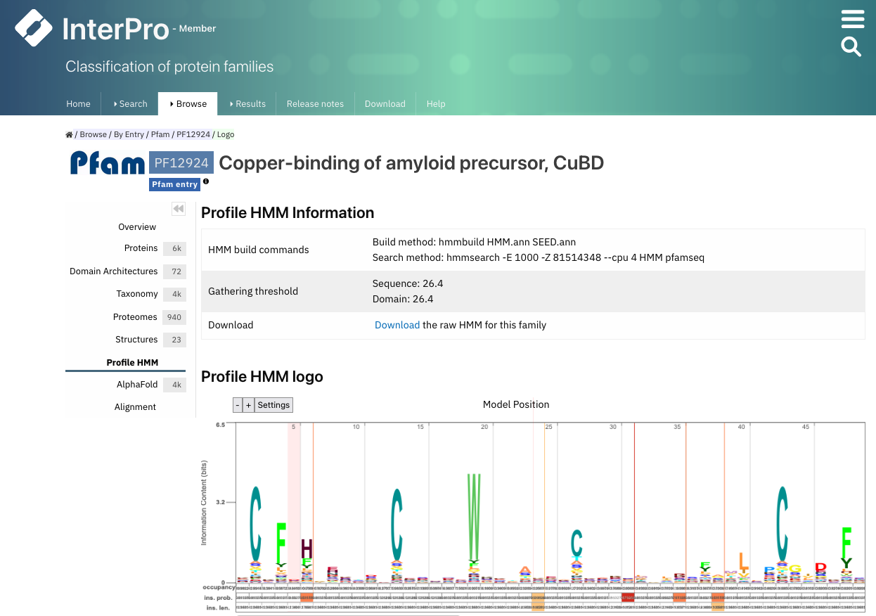
Figure 29:The Pfam logo for PF12924. Credits: Paysan-Lafosse et al. (2022).
File formats
There are many different formats for biological data. A format is a set of rules about the contents and organization of the data. You should be familiar with a couple of common data formats in bioinformatics (See Table 2), which you will experience in the practicals.
Table 2:Examples of common data formats in bioinformatics. Unless explicitly noted these are plain text formats.
| File format | Usage | Common extension |
| FASTA | Nucleotide or amino acid sequences | .fa, .fasta, .fna, .faa |
| Genbank | Sequences, annotations, metadata | .gb |
| Generic Feature Format | Sequence annotations | .gff |
| FASTQ | DNA sequencing data including basecalling quality scores | .fq |
| SAM/BAM (Sequence/Binary Alignment and Map) | Typically alignments between raw sequencing data and a reference, with quality scores | .sam (.bam for the binary file format) |
| VCF (Variant Call Format) | (Genetic) variant calls based on sequencing data aligned to a reference | .vcf (.bcf for the binary file format) |
| PDB | Protein structure data | .pdb |
| Unstructured text | Miscellaneous | .txt |
Plain text files
Many of the biological data formats are plain text files: they only contain letters, numbers, and symbols, but no formatting, such as font size or colors.
Whereas these filetypes can have various different extensions (e.g. .fasta, .gff, etc.), they only contain plain text.
The advantage of plain text files is that they can be opened with any text editor on any computer.
Plain text differs from rich text format, where the latter can also include formatting.
Many bioinformatics programs expect plain text files as input.
Thus, when creating them on your computer, take care to save in this format, and not for example in rtf or word.
On a Windows computer, plain text files can for example be created with the Notepad program (Figure 30).
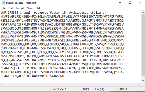
Figure 30:A screenshot of Notepad on Windows. Credits: CC BY-NC 4.0 Ridder et al. (2024).
On a Mac, plain text files can for example be created with the TextEdit program (Figure 31). Take care to set the settings to plain text.
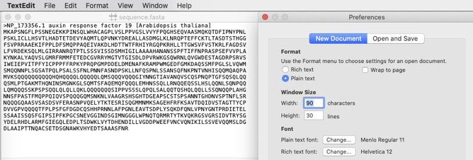
Figure 31:A screenshot of TextEdit on Mac. Credits: CC BY-NC 4.0 Ridder et al. (2024).
There are some important file formats in bioinformatics.
A fasta file stores a DNA or protein sequence (Figure 32).
Information on the sequence is found in the header (starting with >), which is on one line and the sequence can go over multiple lines.
A multi-fasta file stores multiple sequences.
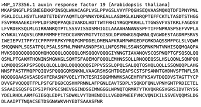
Figure 32:A sequence in fasta format. Credits: CC BY-NC 4.0 Ridder et al. (2024).
The GenBank file format is a popular format to represent genes or genomes. Here you can find an example GenBank record with annotations. Important elements are the Locus, Definition (i.e., the name), and the Organism. Additionally, Features, such as genes and CDSs (coding sequences) are listed.
Binary files
Binary files are all the files that are not text files, they cannot be opened in a text editor.
Instead, they need special programs to write and to open and interpret them.
Examples are word files (.docx) which can be opened with Word, pdf files (.pdf) which can be opened with Acrobat Reader, or image files (e.g., .png) which can be opened with image viewers.
Binary files are are also sometimes used in bioinformatics. Examples include the bam format, which is a binary version of the sam format or the gzip format. Gzip is used for compressing text files without the loss of information. For large files, lots of disk space can be saved this way.
Ontologies
An ontology is a comprehensive and structured vocabulary for a particular domain, such as biology, genetics, or medicine. It defines the various terms used in a domain, along with their meanings and interconnections. As such, ontologies serve as standardized frameworks for organizing and categorizing information in a way that enables effective communication and reasoning among researchers, practitioners, and computer systems. For example, the terms in an ontology can encompass biological entities like genes, proteins, and cells, as well as processes, functions, and interactions that occur within living organisms. Most of the databases mentioned mentioned in this chapter use ontologies in some way to describe their data.
Ontologies play a crucial role in bioinformatics because they facilitate:
- Standardization and consistency: ontologies provide a common language and consistent framework for researchers and professionals, ensuring that everyone understands and uses terms in the same way.
- Interoperability: ontologies facilitate the sharing and integration of data and knowledge across different research groups, institutions, and databases. They enable computer systems to process data more accurately, leading to more meaningful analyses and discoveries.
- Scientific reasoning: by organizing information in a logical and structured way, ontologies help researchers generate hypotheses, design experiments, and validate findings more effectively.
Ontologies typically form a hierarchy, where specific terms point to more generic terms. More generally, most ontologies are represented as a graph, where ontology terms are the nodes and relationships between terms are edges. As such, one ontology term may have more than one parent term. A variety of ontologies are frequently used in the life sciences, some of which are discussed in greater detail below.
Gene Ontology
The Gene Ontology (GO) is a knowledgebase for the function of genes and gene products (e.g. proteins). It is organised into three different domains covering various aspects:
- Molecular Function: molecular-level functions performed by gene products (e.g. proteins), such as ‘catalysis’ or ‘transport’. Most molecular functions can be performed by individual gene products, but some functions are performed by complexes consisting of multiple (possibly differing) gene products. GO molecular functions often include the word “activity” (an amylase enzyme would have the GO molecular function amylase activity).
- Cellular Component: the cellular structures (or location relative to them) in which a gene product performs its function. Can be cellular compartments (e.g., mitochondrion) or macromolecular complexes of which they are part (e.g., the ribosome).
- Biological Process: the larger biological programs composed of multiple molecular activities, for example DNA repair or signal transduction.
A good example of how ontologies are represented as graphs is the biological process hexose biosynthetic process, which has two parents: hexose metabolic process and monosaccharide biosynthetic process. This reflects that biosynthetic process is a subtype of metabolic process and a hexose is a subtype of monosaccharide. (Figure 33).
Edges between GO terms in the GO hierarchy can represent various relationships between genes and gene products. The four main relationship types used in the gene ontology are ‘is a’, ‘part of’, ‘has part’, and ‘regulates’ (see Figure 34).
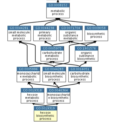
Figure 33:An extract of the Gene Ontology hierarchy. Credits: Binns et al. (2009)
Sequence Ontology
The Sequence Ontology (SO) describes biological sequence elements such as genes or repeats, along with their features and attributes.
The sequence ontology is organized on four main levels:
- Attribute: an attribute describes a certain quality of a given sequence, for example the sequence source (i.e., how it was generated).
- Collection: multiple discontiguous sequences together, for example the chromosomes of a complete genome.
- Feature: the most general top-level entry that describes any extent of a continuous biological sequence, for example a gene is a region, which in turn is a sequence feature.
- Variant: intended to describe genetic variation. The definition of a sequence variant is composed of other entries in the sequence ontology: “A sequence_variant is a non-exact copy of a sequence_feature or genome exhibiting one or more sequence
_alterations”
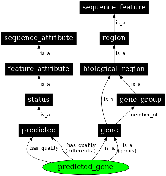
Figure 34:An extract of the Sequence Ontology hierarchy. Credits: Eilbeck et al. (2005).
Other ontologies
Many more ontologies exist and are relevant to biomedical research. The European Bioinformatics Institure (EBI) provides an ontology lookup service that facilitates searching for ontologies. Examples of other ontologies are the plant ontology that describes various anatomical structures in plants, and the human disease ontology.
Practical assignments
This practical contains questions and exercises to help you process the study materials of Chapter 1. You have 2 mornings to work your way through the exercises. In a single session you should aim to get about halfway through this guide (i.e., day 1: assignment 1-3, day 2: assignment 4 and project preparation exercise). Use the time indication to make sure that you do not get stuck in one assignment. These practical exercises offer you the best preparation for the project. Especially the project preparation exercise at the end is a good reflection of the level that is required to write a good project report. Make sure that you develop your practical skills now, in order to apply them during the project.
Note, the answers will be made available after the practical!
Glossary
- Annotation
- The process of identifying functional elements within a genomic sequence, such as genes, coding regions, and regulatory motifs.
- Cell
- The basic structural and functional unit of all living organisms.
- DNA
- DeoxyriboNucleic Acid
- Exon
- A DNA segment in a gene that encodes part of the mature messenger RNA (mRNA) after intron removal.
- Gene
- A segment of DNA that encodes functional products, typically proteins.
- Genome
- The complete set of genes or genetic material present in a cell or organism.
- Genome browser
- A tool for visually inspecting genomic regions, annotations, and experimental data tracks.
- HMM
- Hidden Markov Model - a statistical model that represents systems where the states are not directly observable (hidden) but can be inferred from observable data.
- Intron
- A DNA segment in a gene that is not expressed in the mature messenger RNA (mRNA) product and is removed during the RNA splicing process.
- mRNA
- Mature mRNA, or mature messenger RNA, is a processed form of RNA that has had its introns removed and consists only of exons, making it ready for translation into proteins.
- miRNA
- MicroRNA are small, single-stranded, non-coding RNA molecules containing 21–23 nucleotides.
- Nucleotide
- The basic building block of DNA and RNA, consisting of a base, sugar, and phosphate group.
- Protein
- A molecule composed of amino acids, encoded by genes, and responsible for cellular structure and function.
- RNA
- RiboNucleic Acid
- rRNA
- Ribosomal RNA is a type of non-coding RNA that is a key component of ribosomes, which are essential for protein synthesis in all living cells.
- Sequence
- The precise order of nucleotides in a DNA or RNA strand.
- Splicing
- A biological process where non-coding regions (introns) are removed from a precursor messenger RNA (pre-mRNA) transcript, and the coding regions (exons) are joined together to form a mature messenger RNA (mRNA) that can be translated into proteins.
- Transcription
- The process of copying a DNA sequence into RNA.
- Translation
- The process of converting RNA sequences into proteins.
- tRNA
- Transfer RNA, is a type of RNA molecule that helps decode messenger RNA (mRNA) sequences into proteins.
- Clark, M. A., Douglas, M., & Choi, J. (2018). 3.5 Nucleic Acids. In Biology 2e. OpenStax. https://openstax.org/books/biology-2e/pages/3-5-nucleic-acids
- OpenStax College. (2013). DNA Nucleotides. https://commons.wikimedia.org/wiki/File:DNA_Nucleotides.jpg
- Ball, M. P. (2013). DNA replication split. https://commons.wikimedia.org/wiki/File:DNA_replication_split.svg
- Koch, L. (2009). Semiconservative replication. https://commons.wikimedia.org/wiki/File:Semiconservative_replication.png
- UC Museum of Paleontology. (2020). The causes of mutations. https://evolution.berkeley.edu/evolution-101/mechanisms-the-processes-of-evolution/the-causes-of-mutations/
- Ridder, D. de, Kupczok, A., Holmer, R., Bakker, F., Hooft, J. van der, Risse, J., Navarro, J., & Sardjoe, T. (2024). Self-created figure.
- miguelferig. (2011). Intron miguelferig. https://commons.wikimedia.org/wiki/File:Intron_miguelferig.jpg
- Greenwood, S. (2018). Genetic Code. https://commons.wikimedia.org/wiki/File:Genetic_Code.png
- Squidonius. (2008). Molbio-Header. https://commons.wikimedia.org/wiki/File:Molbio-Header.svg
- Clark, M. A., Douglas, M., & Choi, J. (2018). 3.4 Proteins. In Biology 2e. OpenStax. https://openstax.org/books/biology-2e/pages/3-4-proteins
- LadyofHats. (2008). Main protein structure levels en. https://commons.wikimedia.org/wiki/File:Main_protein_structure_levels_en.svg
- OpenStax College. (n.d.). Protein Structure. https://openstax.org/books/microbiology/pages/7-4-proteins#OSC_Microbio_07_04_secondary
- Laskowski, R. A., MacArthur, M. W., Moss, D. S., & Thornton, J. M. (1993). PROCHECK: a program to check the stereochemical quality of protein structures. Journal of Applied Crystallography, 26(2), 283–291. https://doi.org/10.1107/S0021889892009944
- Sangrador, A. (2023). What are protein domains? https://www.ebi.ac.uk/training/online/courses/protein-classification-intro-ebi-resources/protein-classification/what-are-protein-domains/
- Berman, H. M., Westbrook, J., Feng, Z., Gilliland, G., Bhat, T. N., Weissig, H., Shindyalov, I. N., & Bourne, P. E. (2000). The Protein Data Bank. In Nucleic Acids Research (Vol. 28, pp. 235–242). 10.1093/nar/28.1.235